Munich Personal RePEc Archive
Is there a direct effect of corruption on
growth?
Dzhumashev, Ratbek
Monash University, Dept. of Economics
9 November 2009
Is there a direct effect of corruption on
growth?
Ratbek Dzhumashev∗
November 9, 2009
Abstract
Recent empirical studies find that the direct effect of corruption on
growth is statistically insignificant. However, there exists a
discrep-ancy between these results and the intuition that corruption reduces
over-all productivity, because total factor productivity also depends
on the quality of institutions and their efficiency. The current
pa-per addresses this issue and offers a new pa-perspective on growth
ef-fects of corruption and shows that direct and indirect growth efef-fects
of corruption can be statistically significant. Moreover, the empirical
results confirm the existence of both negative and positive growth
effect of corruption.
1
Introduction
Recent empirical studies find that the direct effect of corruption on growth
is statistically insignificant. This finding is inconsistent with the notion
of overall productivity deterioration due to corruption, because the total
factor productivity also depends on the quality of institutions and their
efficiency. This paper addresses this issue and offers a new perspective
on modeling the growth effects of corruption and finds that the direct
effect of corruption on growth is statistically significant.
In his seminal paper, Mauro (1995) finds some support for a
nega-tive relationship between growth and the bureaucratic efficiency index
∗Dept. of Economics, Monash University, 100 Clyde Rd, Berwick, 3805, Australia.
and the corruption index. By running various regressions of per capita
GDP growth on bureaucratic efficiency or the corruption index, he shows
that this relationship is robust for bureaucratic efficiency, however, not
for the corruption index. Nevertheless, Levine and Renelt (1992) show
empirically that the investment rate is a robust determinant of economic
growth. Taking that into account, Pelegrini and Gerlagh (2004) find that
after controlling for investment, the effect of corruption in à la Mauro
(1995) specification becomes insignificant. Moreover, Barro and
Sala-i-Martin (2004) report that estimation based on the indicator from the
In-ternational Country Risk Guide (ICRG) on the extent of official corruption
and the indicator for the quality of the bureaucracy, have insignificant
effects on growth. Supporting these results, Dreher and Herzfeld (2005),
Pelegrini and Gerlagh (2004), and Everhart et al. (2009), find that the direct effect of corruption appears insignificant with respect to growth
in GDP per capita. On the other hand, the indirect effect of corruption
working through public investment and quality of governance (e.g. Mo, 2001 and Everhartet al., 2009), and investment and trade openness (e.g.
Pelegrini and Gerlagh, 2004) is significant.
These empirical results, which suggest that corruption may not have
a significant direct impact on growth, are likely to stem from
theoreti-cal vagueness. Notably, there are some gaps in theoretitheoreti-cal approaches,
which relates corruption to growth rates. It is well known that
corrup-tion distorts the public-private interaccorrup-tions, and hence, the effect of the
public sector on economic growth is altered.1 However, in growth
stud-ies, corruption has not been modeled as a factor that changes the overall
effect of the public sector on economic activity. It is rather captured by
its partial effects. For example, Mauro’s (2002) model incorporates
in-efficiency of the public sector as misuse of public funds, which leads to
lower productive public inputs to aggregate production. Although, the
effect of corruption on public sector burden has not been accounted for.
In a similar manner, in Blackburn et al. (2002), corruption is modeled as
bribe-taking from tax-evaders, while in Blackburn et al (2005), corruption
1
is manifested as embezzlement of public funds.2 There are also models
that relate corruption to overall productivity. For example, Mo (2001) and
Everhartet al.(2009) provide models that capture the direct effect of cor-ruption on growth through the rate of productivity growth. However, in
these models, the indirect effect of corruption is not formulated explicitly.
Unlike the existing studies, this paper provides a simple theoretical
model that incorporates both indirect and direct effect of corruption on
growth. The indirect effect is transmitted via an overall distortion of the
impact of the public sector on economic activity and through reduced
investment demand. The direct effect works through the change in the
total factor productivity, due to corruption. This approach to modeling
corruption is presented in the next section. Further, I test the
implica-tions of the model using dynamic panel data estimators. This estimation
method is more suitable to panel data with a short time horizon and
per-sistence in time series.3
2
A simple model with corruption in the public
sector
Traditionally, the public sector is modeled as a productive externality
pro-vided to private producers by the government which comes at the cost of
private disposable income decreased by taxes. Arrow and Kurz (1970)
and Barro (1990) incorporated public sector services directly into the
production function as follows: y = f(k, g), where k is capital stock per
worker, andg is the productive externality of government expenditure in
per worker terms. To finance the productive public input, g, private
pro-ducers have to pay taxes, and hence, their income, net of taxes, is given
as(1−τ)y.This is the case in general, regardless of whether corruption
ex-ists in the public sector. However, corruption makes the effective burden
of taxes, τ, deviate from the statutory one. The productive externality
2See also Mauro,1998; Tanzi, 1998; Barreto, 2000; Keefer and Knack, 2002; Del Monte
and Papagni, 2001; Lambsdorff, 2003; Meon and Weill, 2006; Delavallade, 2006; De la Croix and Delavallade, 2009.
provided by government,g, can also be altered by corrupt behavior of the
bureaucrats. The resulting distortions in the cost and benefit of the
pub-lic sector caused by corruption leads to a change of the marginal product
of private capital. Therefore, corruption affects investment through
dis-tortions in private capital productivity. To be more specific, I assume that
production at timetis given by:4
Yt=KαGβt(AtLt)1−α−β (1)
It is assumed that the overall productivity evolves according to the
func-tion:
At=A0eςt, (2)
where ς is the growth rate of productivity (or technology). Denoting by
i , the fraction of income invested into physical capital and expressing
output and stock of capital in per unit of effective labour, the equation
describing the evolution of physical capital stock is written as:
˙ˆ
kt=iyˆt−(n+ς+δ)ˆkt (3)
where yˆ = Y/AL = ˆkαgˆβ is output per unit of effective worker, ˆk = K/AL is
capital stock per unit of effective worker,gˆ=G/ALis government
expen-diture per unit of effective worker, andnis a constant population growth
rate, andς is a constant technology growth rate.
A steady-state value of capital is found from (3):
ˆ
k∗ =
iˆgβ n+ς+δ
1−1α
.
By inserting the expression for steady state capital above back into (1)
and taking logs, steady state income per capita is derived as:
lnyˆ∗
t =
β
1−αlnˆgt+ α
1−αln i
∗− α
1−αln(n+ς+δ) (4)
This is the well-known empirical growth equation used by Mankiw et al.
4It is also possible to consider the production function similar to Mankiw et al. (1992)
given asYt=AtKtαG β tH
ϕ tL
ϑ
(1992). However, they employed cross-section data for estimations, hence,
they were not concerned about the dynamics of the growth process.
Islam (1995) has shown how to adjust this model for the panel data
framework. I follow his approach and derive a dynamic panel data model.
This is done by approximating the pace of convergence around the steady
state level of output, yˆ∗. This leads to the expression of the adjustment
process around the steady state:
lnyˆt= (1−e−λ)(lnyˆ∗−e−λlnyˆt−1).
whereλ = (n+ς+δ)(1−α). After some rearrangement and substitution
foryˆ∗ from (4), we arrive at:
lnˆyt−lnˆyt−1 = (1−e−
λ)[ β
1−αlnˆgt+ α
1−αln i− α
1−αln(n+ς+δ)−lnyˆt−1]. (5)
By noting that
lnyˆt=ln yt−ln A0−ςt,
whereyt=Yt/Lt, (5) is transformed into the following form:
ln yt= (1−e−λ)[
β
1−αln gt+ α
1−αln i− α
1−αln(n+ς+δ) + (6)
+1−α+β
1−α lnA0] +e −λln y
t−1+ς
t(1−α−β)(1−e−λ)
1−α +e −λ
How should corruption be incorporated into this result? As it was
dis-cussed above, corruption affects the public input, g, and the investment
level, i. By affecting the technology coefficient, A, corruption can also
impact growth directly. I employ this rationale to incorporate corruption
into this growth model.
Let us first consider how corruption influences the technology
coeffi-cient, At. Since the productivity gains from any technology are likely to
be lower for countries with higher corruption, it is reasonable to assume
that corruption affects the level of technology, At. Based on the idea
that corruption not only directly lowers productivity but also dampens it
im-pact of corruption on productivity grows at an increasing rate. Thus, the
evolution of technology, given by (2), is modified to:
At=
A0eςt,
eχ (7)
where 0 < χ < χ¯ stands for the coefficient that measures corruption, so
when χ = 0, there is no corruption, whereas χ¯ stands for the maximum
value for the corruption measure.
Next, let us consider how corruption distorts the economic effect of
the public sector. Intuitively it is clear that corruption makes the
pub-lic sector inefficient. This generally means that for a given tax revenue,
the government generates less amount of productive inputs. Therefore,
the public productive input, in a very simple case, can be expressed as:
g= f(χ)τ y , withτ ybeing the total tax revenue in per capita terms, and f(χ)
is an increasing function of the level of corruption. However, corruption
distorts the collection of taxes, and ultimately the output level is also
endogenous and influenced by corruption. To capture this complex
rela-tionship, one can express the public inputs as a function of the average
tax rate,τ , output, yt, and the level of corruption: gt=g(τ, yt, χ).
Finally, corruption affects investment through increased uncertainty
and reduced productivity.5 Uncertainty requires an additional premium
on investment returns, hence, it raises real interest rates, and leads to
lower investment demand. Public inputs into production are reduced by
corruption, which, in turn, decreases private capital productivity. To
cap-ture this idea, one can write the amount of investment as the following
function:
it=i[rt(χ)] (8)
wherertis the real interest rate, which itself is an increasing function of
corruption. In our contextr′t(χ)>0andi′t(χ)<0.
Now, based on the discussion above, the growth equation given by (6)
can be modified to incorporate the effects of corruption. The modification
5See Lambsdorff, 2003; Campos, 2001; Shleifer and Vishny, 1993; Aizenman and
yields:
ln yt= (1−e−λ)[
β
1−αln gt(τ, yt, χ) + α
1−αln i(χ)− α
1−αln(n+ς+δ) +
+1−α+β
1−α lnA0−
1−α+β
1−α χ] +e −λln y
t−1+ς
(1−α−β)(1−e−λ)
1−α +e −λ
(9)
Equation (9) expresses the direct and indirect influence of corruption
on the evolution of per capita output over time. Corruption directly
af-fects per capita output, decreasing the technology growth rate.
Corrup-tion also indirectly influences per capita output growth by reducing the
growth of private capital and diminishing the productive externality
pro-vided by the public sector. Using the conventional notation of the panel
data literature, (9) is rewritten as follows:
zit=γzi,t−1+
4
X
j=1
βjxjit+ηt+µi+υit, (10)
wherezit=ln yt,zi,t−1 =ln yt−1,γ =e−
λ,β
1 = (1−e−λ)1−βα,β2 = (1−e−λ)1−αα,
β3 = −(1−e−λ)1−αα, β4 = −(1−e−λ)1−1−α+βα , x1it = ln gt(τ, yt, χ), x2it = ln i(χ),
x3
it =ln(n+ς+δ),xit4 =χ,ηt= (1−α−β)(1−e
−λ)
1−α , andµi= (1−e
−λ)1−α+β
1−α lnA0+ςe.
This modeling approach has several advantages over the models used
in the literature: i) importantly, it builds on the well known neoclassical
growth model; ii) the model allows the use of the dynamic panel data
methods in estimations; iii) in addition, incorporation of the effects of
cor-ruption into the model is done in a general way that captures main direct
and indirect effect of corruption. The assumptions in modeling are based
on the stylized facts, suggested by the empirical and theoretical research
mentioned above. Now, in the next section, we turn to the discussions of
an empirical model based on equation (10).
2.1 The estimation method
To obtain the empirical specification used for estimations, I have made
some adjustments to the model given by (10). To capture the effect of
corruption on investment and public services, I have included the
input, log(git) and between the level of corruption, corruptionit), and log
of investment, log(iit). In addition, I include other conditioning variables
given by a vector:
Z ={log(git), log(sch2it), log(Iit/Nit), developmentit}, wheresch2is a measure
of secondary school enrollment, I/N is the amount of private investment
per capita,developmentis a measure of economic development as GDP per
capita or the quality of public institutions.6 After incorporating all
adjust-ments mentioned above, the resulting empirical model to be estimated
is written as:
log(yit) =αt+γi+β0log(yit−1) +β1(corruptionitlog(g)it) +
+β2(corruptionitlog(i)it) +β3corruptionit+β4Zit+εit (11)
It should be noted that one might encounter several difficulties related
to estimation of equation (11):
• corruption is endogenous as economic growth and corruption may
cause each other, thus,corruptionit may be correlated with the error
term;
• the explanatory variables may be correlated with country-specific
fixed effects, thus causing the error term to be correlated with the
explanatory variables;
• the lagged dependent variablelog(yit−1)on the right-hand side may
lead to auto-correlation of the error term;
• the panel dataset has a short time dimension that contributes to
estimation bias.
These estimation issues can be overcome by using Arrelano-Bond (1991)
Difference GMM estimators and Blundell-Bond (1998) System GMM
esti-6In the estimations, I used as a measure of the quality of institutions, the Economic
mators. Arrelano-Bond estimator (Difference GMM) uses the lagged level
endogenous variables as instruments. In case, the dependent variable is
close to a random walk, the Difference GMM estimator may not be
effi-cient because past levels convey little information about future changes,
that makes lagged levels of the regressors poor instruments for the
dif-ferenced regressors.7 Therefore, equation (11) is estimated using the
Blundell-Bond (1998) System GMM estimator. It is also known that the
system estimators have a downward bias due to smaller SEs of the
es-timates, when cross-section dimension is small. This may lead to false
significance of the regressors.8 Windmeijer’s (2005) procedure that
al-lows to compute heteroskedasticity-consistent SEs is used to correct this
bias.9 Consistency of the System GMM estimator depends on the validity
of the instruments. To see if the the instruments are valid, the Hansen
test for over-identifying restriction is utilized. In addition, the first and
second order autocorrelation test for the error term is performed. The
AR(1) and AR(2) statistics are used to test the null of no autocorrelation.
The test results are reported in Table 1 and 2, in section 2.3.
2.2 Data description
The dataset used in estimations covers the time period from 2000 to 2007
across 141 countries.
Corruption measures: As measures of corruption, after some
trans-formation, I use the Corruption Perception Index (CPI) complied by the Transparency International, and the Control of Corruption Index (CC) from Governance Indicators Dataset complied by the World Bank (Kaufmann et
al., 2004; Kaufmann, 2004). The CPI values are determined in the range
of (0,10); the higher the value, the less there is corruption in the
econ-omy. The Control of Corruption Index, CC, ranges within (-1.5, 2.8), and again higher values indicate lower corruption. Since, these measures are
counterintuitive, I convert them into intuitive measure of corruption by
using the following procedure: first, normalize the original lack of
cor-7See Temple et al. (2001), Roodman (2006). 8See Judson and Owen (2000).
9
ruption measures as, CP I = max(CP ICP I ) and CC = max(CC)CC , then I use, as a
measure of corruption,(1−CP I) and(1−CC).
Control variables: As a proxy for the quality of public institutions,
I use the Index of Business Regulations (busreg).The data on this index
come from the Fraser Institute. This index captures the burden on the
private agents due to price controls, administrative procedures and other
obstacles that hinder starting a new business, time cost of senior
man-agement in dealing with government bureaucracy, payments or bribes
such as irregular, additional payments connected with permits, licenses,
exchange controls, tax assessments, and police protection. The higher
values of this index signify public institutions which are of a higher
qual-ity.
As control variables, I also use GDP per capita in constant $US, (Y/N), secondary gross enrollment rates, (SCH2), government size, (G/Y), and physical capital investment, (I/Y). The data on GDP per capita,G/Y, SCH2, andI/Y are obtained from the World Bank database: the World Develop-ment Indicators.
2.3 Results and discussion
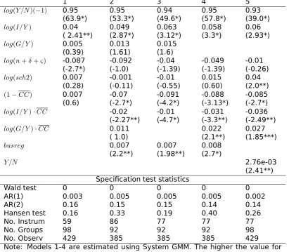
It is notable, that without the interaction terms in the specification, the
direct effect of corruption is not significant for both measures of
corrup-tion. It is likely that the existing empirical results, which find the direct
growth effect of corruption statistically insignificant, are driven by the
bias caused by omission of the indirect effects of corruptions in
estima-tions. However, in specifications when at least one of the indirect
chan-nels is accounted for, the direct effect of corruption proves to be
statis-tically significant and of the right sign. Therefore, we can conclude that
corruption is a significant negative factor for economic growth.
The results show that the effects of public sector inputs,log(G/Y), are insignificant in all estimations. Although, the coefficient on the
interac-tion term between lack of corrupinterac-tion and public spending is positive and
statistically significant in most cases. This confirms our theoretical
Table 1: Estimation results. Corruption measure: the Control of Corrup-tion Index
1 2 3 4 5
log(Y /N)(−1) 0.95 0.95 0.94 0.95 0.93
(63.9*) (53.3*) (49.6*) (57.8*) (39.0*)
log(I/Y) 0.04 0.049 0.063 0.058 0.06 ( 2.41**) (2.87*) (3.12*) (3.3*) (2.93*)
log(G/Y) 0.005 0.013 0.015 (0.39) (1.61) (1.6)
log(n+δ+ς) -0.087 -0.092 -0.04 -0.049 -0.01 (-2.7*) (-1.0) (-1.39) (-1.39) (-0.26)
log(sch2) 0.007 -0.001 -0.01 0.015 0.04 (0.28) (-0.11) (-0.55) (0.60) (2.0**)
(1−CC) 0.007 -0.07 -0.091 -0.088 -0.085 (0.6) (-2.7*) (-4.2*) (-3.13*) (-2.7*)
log(I/Y)·CC -0.02 -0.01 -0.031 -0.036 (-2.27**) (-4.7*) (-3.3**) (-2.49**)
log(G/Y)·CC 0.011 0.022 0.027
( 1.0) (2.1**) (1.85***)
busreg 0.007 0.007 0.008
(2.2**) (1.98**) (2.7*)
Y /N 2.76e-03
(2.41**) Specification test statistics
Wald test 0 0 0 0 0
AR(1) 0.003 0.005 0.005 0.005 0.002
AR(2) 0.16 0.15 0.15 0.14 0.14
Hansen test 0.16 0.33 0.19 0.40 0.26
No. Instrum 59 86 77 77 77
No. Groups 98 92 92 92 98
No. Observ 429 385 385 385 429
Note: Models 1-4 are estimated using System GMM. The higher the value for
CC, the higher is corruption. In parenthesis, heteroskedasticity-consistent with finite-sample Windmeijer (2005) correction, t-statistics are reported. (*), (**), and (***) denote statistical significance at 1%, 5%, and 10% level, correspond-ingly. The Wald test tests for the joint-significance of all coefficients included in the regression and is distributed asχ2 with degrees of freedom equal to the
number of restrictions. The Hansen test is used to test the null hypothesis that the instruments are valid. This statistics is distributed as χ2 with degrees of
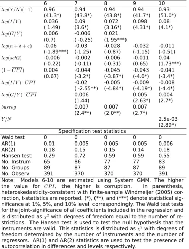
Table 2: Estimation results. Corruption measure: the Control Perception Index
6 7 8 9 10
log(Y /N)(−1) 0.96 0.94 0.94 0.94 0.93
(41.3*) (43.8*) (43.8*) (41.7*) (51.0*)
log(I/Y) 0.036 0.09 0.072 0.098 0.08 ( 1.49) (3.6*) (3.16*) (4.31*) (4.1*)
log(G/Y) 0.006 -0.006 0.021 (0.7) ( -0.25) (1.95***)
log(n+δ+ς) -0.06 -0.03 -0.028 -0.032 -0.011 (-1.89***) (-1.25) (-0.87) (-1.15) (-0.51)
log(sch2) -0.006 -0.002 -0.006 -0.011 0.04 (-0.22) (-0.11) (-0.31) (0.65) (1.73***)
(1−CP I) 0.004 -0.044 -0.045 -0.043 -0.041 (0.67) (-3.2*) (-3.87*) (-4.0*) (-3.4*)
log(I/Y)·CP I -0.02 -0.005 -0.009 -0.008 ( -2.55**) (-4.84*) (-4.19*) (-4.4*)
log(G/Y)·CP I 0.006 0.005 0.004 (1.44) (2.63*) (2.7*)
busreg 0.007 0.007 0.007
(2.4**) (2.0**) (2.7*)
Y /N 2.5e-03
(2.89*) Specification test statistics
Wald test 0 0 0 0 0
AR(1) 0.01 0.005 0.005 0.005 0.006
AR(2) 0.18 0.15 0.15 0.14 0.18
Hansen test 0.29 0.72 0.59 0.59 0.55
No. Instrum 65 86 77 77 83
No. Groups 89 87 87 87 89
No. Observ 391 370 370 370 391
Note: Models 6-10 are estimated using System GMM. The higher the value for CP I, the higher is corruption. In parenthesis, heteroskedasticity-consistent with finite-sample Windmeijer (2005) cor-rection, t-statistics are reported. (*), (**), and (***) denote statistical sig-nificance at 1%, 5%, and 10% level, correspondingly. The Wald test tests for the joint-significance of all coefficients included in the regression and is distributed asχ2 with degrees of freedom equal to the number of
re-strictions. The Hansen test is used to test the null hypothesis that the instruments are valid. This statistics is distributed asχ2 with degrees of
the public sector, and hence, negatively affects overall economic
perfor-mance.
The estimations confirm the positive growth effects of physical capital
investment. Curiously, the interaction term between the lack of
corrup-tion measure (CCorCPI) and investment has a negative coefficient. This result is capturing the positive effect of corruption on investment through
a decrease in red tape and regulatory burden.
The estimation results also suggest that human capital accumulation,
log(sch2) is not significant, unless the per capita income level is con-trolled for. The results also confirm that the quality of institutions
(ex-pressed by the Index of Business Regulations,busreg) plays a significant positive role in economic growth. It is likely that the stock of human
cap-ital is instrumental to growth only when the environment is less corrupt
and the quality of the institutions is high.
Another difference of these estimation results from the existing ones is
that the term,log(n+δ+ς), is insignificant overall, although the sign of the
coefficient is correct. Only when the interaction terms with lack of
corrup-tion are omitted, the effect of this term becomes significant. The possible
explanation is that when the interaction between investment and
corrup-tion (or lack of it) is included in the specificacorrup-tion, the assumpcorrup-tion that the
rate of technology growth,ς, and the rate of depreciation,δ, is the same
across the countries, is not valid anymore. Hence, the impact of these
three parameters becomes blurred and insignificant.
The overall effect of corruption is negative, as the negative effects
transmitted directly and through the public sector inefficiencies
domi-nate the positive effect through increased investment, which is possibly
caused by collusive corruption that allows the firms to overcome
exces-sive red tape and the burden of regulations.
3
Conclusion
By using a model that treats corruption as distortions created in the
it has been shown how corruption affects growth directly and indirectly.
Empirical estimations confirm that corruption can affect growth in both
ways. This result differs from the previous findings in that even after
con-trolling for the effect of corruption through investments and public sector
inputs, there is evidence of an overall direct negative effect. From this
re-sult one can infer that corruption inhibits growth by distorting the publicly
provided productive externality and by deteriorating the overall business
climate and perpetuating bad expectations about economic
opportuni-ties. However, the results also indicate that investment levels are higher
with an increase in corruption levels, other things being equal. Therefore,
the model presented in the paper is able to capture both negative and
positive effects of corruption on growth simultaneously. Nevertheless,
the overall effect of corruption is negative, as the negative effects
trans-mitted directly and through the public sector inefficiencies are greater
than the positive effect through investment.
References
Aizenman, J. and N. Marion (1993). Policy uncertainty, persistence, and growth. Review of International Economics 1, 145–163.
Angeletos, G.-M. (2007). Uninsured idiosyncratic investment risk and ag-gregate saving. Review of Economic Dynamics 10, 1–30.
Arellano, M. and S. Bond (1991). Some tests of specification for panel data: Monte carlo evidence and application to employment equations.
Review of Economic Studies 58, 277–97.
Arrow K. and M. Kurz (1970). Public investment, the rate of return and optimal fiscal policy. The Johns Hopkins University Press, Baltimore. Barreto, R. A. (2000). Endogenous corruption in a neoclassical growth
model. European Economic Review 44(1), 35–60.
Barro, R. J. (1990). Government spending in a simple model of endoge-nous growth. The Journal of Political Economy 98(5 Part 2), S103–S125. Barro, R. J. and X. Sala-i-Martin (2004). Economic Growth. MIT Press. Blackburn, K., N. Bose, and M. E. Haque (2005). Public Expenditures,
Bureaucratic Corruption and Economic Development. The University of Manchester, Centre for Growth and Business Cycle Research, DPS 053.
Blundell, R. and S. Bond (1998). Initial conditions and moment restrictions in dynamics panel data models. Journal of Econometrics 87, 115–143. Campos, J. E. L. (2001). Corruption : the boom and bust of East Asia.
Quezon City: Ateneo de Manila University Press.
De la Croix, D. and C. Delavallade (2009). Growth, public investment and corruption with failing institutions. Economics of Governance 10, 187–219.
Delavallade, C. (2006). Corruption and distribution of public spending in developing countries. Journal of Economics and Finance 30(2), 222– 239.
Del Monte, A. and E. Papagni (2001). Public expenditure, corruption, and economic growth: the case of Italy. European Journal of Political Econ-omy 17, 1–16.
Dreher, A. and T. Herzfeld (2005). The economic costs of corruption: a survey and new evidence. Working Paper, Thurgau Institute of Eco-nomics, Kreutzlingen, Switzerland.
Everhart, S. S., Vazquez, J. M. and R. M. McNab (2009). Corruption, gov-ernance, investment and growth in emerging markets. Applied Eco-nomics 41(13), 1579–1594.
Galtung, F. (2006) Measuring the Immeasurable: Boundaries and Func-tions of (Macro) Corruption Indices, in Measuring Corruption, C. Samp-ford, A. Shacklock, C. Connors, and F. Galtung , Eds. Ashgate, 101-130.
Islam, N. (1995). Growth empirics: a panel data approach. Quarterly Journal of Economics 110, 1127–70.
Judson, R. and A. Owen (1999). Estimating dynamic panel data models: a guide for macroeconomists. Economics Letters 65, 9–15.
Kaufmann, D., A. Kraay, and M. Mastruzzi (2004). Measuring Governance Using Cross-Country Perceptions Data. Washington DC.: World Bank.
Kaufmann, D.(2004). Corruption, Governance and Security:
Challenges for the Rich Countries and the World, Chap-ter in the Global Competitiveness Report 2004/2005 -www.worldbank.org/wbi/governance/pubs/gcr2004.html
Keefer, P. and S. Knack (2002). Rent-seeking and Policy Distortions when Property Rights are Insecure. Working paper 2910. The World Bank. Lambsdorff, J. G. (2003). How corruption affects productivity.
KYK-LOS 56(4), 457–474.
Levine, R. and D. Renelt (1992). A Sensitivity Analysis of Cross-Country Growth Regressions. American Economic Review 82(4), 942–63.
Mankiw, G., D. Romer, and D. Weil (1992). A contribution to the empirics of economic growth. Quarterly Journal of Economics 107, 407–37. Mauro, P. (1995). Corruption and growth. Quarterly Journal of
Mauro, P. (1998). Corruption and the composition of government expen-diture. Journal of Public Economics 69(2), 263–279.
Meon, P.-G. and L. Weill (2006). Is corruption an efficient grease? A cross-country aggregate analysis. InPublic Choice Conference 2006, Amster-dam.
Mo, P. H. (2001). Corruption and economic growth.Journal of Comparative Economics 29(1), 66–79.
Naudé, W.A. and W. F. Krugell (2007). Investigating geography and in-stitutions as determinants of foreign direct investment in Africa using panel data. Applied Economics 39(10), 1223–1233.
Pellegrini, L. and R. Gerlagh (2004). Corruption’s effect on growth and its transmission channels. KYKLOS 57(3), 429–456.
Romero-Avila, D. (2008). Productive physical investment and growth: testing the validity of the AK model from a panel perspective. Applied Economics 40(1), 1–17.
Roodman, D. (2006). How to Do xtabond2: An Introduction to "Differ-ence" and "System" GMM in Stata. Working Paper 103. Center for Global Development, Washington.
Sepulveda, F. and F. Mendez (2006). Corruption, growth and political regimes: Cross country evidence. European Journal of Political Econ-omy 22(1), 82–98.
Shleifer, A. and R. W. Vishny (1993). Corruption. The Quarterly Journal of Economics 108(3), 599–617.
Sik, Endre (2002). The Bad, the Worse and the Worst: Guesstimating the Level of Corruption,, in Political Corruption in Transition: A Skeptic’s Handbook, Stephen Kotkin and Andras Sajo, Eds. Budapest: Central European University Press, 91-113.
Tanzi, V. (1998). Corruption around the world - causes, consequences, scope, and cures.International Monetary Fund Staff Papers 45(4), 559– 594.
Temple, J., S. Bond, and A. Hoeffler (2001). GMM estimation of empirical growth models CEPR Discussion Paper 3048, London School of Eco-nomics.