http://dx.doi.org/10.4236/ojs.2016.62025
How to cite this paper: Jere, S. and Moyo, E. (2016) Modelling Epidemiological Data Using Box-Jenkins Procedure. Open Journal of Statistics, 6, 295-302. http://dx.doi.org/10.4236/ojs.2016.62025
Modelling Epidemiological Data Using
Box-Jenkins Procedure
Stanley Jere
*, Edwin Moyo
Department of Mathematics and Statistics, Mulungushi University, Kabwe, Zambia
Received 27 November 2015; accepted 23 April 2016; published 26 April 2016
Copyright © 2016 by authors and Scientific Research Publishing Inc.
This work is licensed under the Creative Commons Attribution International License (CC BY). http://creativecommons.org/licenses/by/4.0/
Abstract
In this paper, the Box-Jenkins modelling procedure is used to determine an ARIMA model and go further to forecasting. We consider data of Malaria cases from Ministry of Health (Kabwe District)- Zambia for the period, 2009 to 2013 for age 1 to under 5 years. The model-building process in-volves three steps: tentative identification of a model from the ARIMA class, estimation of para-meters in the identified model, and diagnostic checks. Results show that an appropriate model is simply an ARIMA (1, 0, 0) due to the fact that, the ACF has an exponential decay and the PACF has a spike at lag 1 which is an indication of the said model. The forecasted Malaria cases for January and February, 2014 are 220 and 265, respectively.
Keywords
Box-Jenkins Modeling Procedure, ARIMA Model, Exponential Decay, Spike
1. Introduction
Malaria remains one of the most causes of human morbidity and mortality with a high rate in Africa and Asia. Reference [1] states that, “the vast majority of cases (81%) were in the African region followed by South-East Asia (13%) and Eastern Mediterranean Region (6%)”. There are indications that malaria represents over 10% of Africa’s overall disease burden. Malaria is mostly common in Africa, where it has remained a serious problem accelerating poverty and hindering economic development. Malaria can result in decreased gross domestic product by as much as 1.3% in countries with high disease rates [2]. In this paper, we discuss the Box-Jenkins modeling procedure to determine an ARIMA model and forecast.
The Box-Jenkins approach to forecasting was first described by statisticians George Box and Gwilym Jenkins and was developed as a direct result of their experience with forecast problems in the business, economic, and control engineering applications [3]. Fitting a time series model using the Box-Jenkins modeling procedure
lows us to determine an ARIMA (p, d, q) model which is simple and provides a sufficiently accurate description of the behavior of the data. To build a reasonable ARIMA model, as a rule of thumb, Box-Jenkins requires at least 40 or 50 equally-spaced periods of data. The data must also be edited to deal with extreme or missing val-ues or other distortions through the use of functions as log or inverse to achieve stabilization. We need a mini-mum of n = 50 observations and a number of ACF and PACF to be calculated should be about n/4. The reason why we calculate the ACF and PACF is to use them in identifying the orders of p and q by matching the patterns with the theoretical patterns of known models. A known shortcoming of Box-Jenkins forecasts is that they are based strictly upon univariate analysis, and this limits its use for exploring relationships to time and number of events [4]. Box-Jenkins forecasting is of greatest use when the underlying factors causing demand for products, services, revenue, and, in this case, disease burden is believed to behave in the future in much the same manner as it did in the past [5].
The application significance of this study is that by developing forecasting models for predicting the expected number of malaria cases in advance, timely prevention and control measures can be effectively planned like eli-minating vector breeding places, spraying insecticides, and creating public awareness.
The model-building process involves three steps.
1) Tentative identification of a model from the ARIMA class. 2) Estimation of parameters in the identified model.
3) Diagnostic checks.
Tentative identification of model—at this stage we use two graphical devices which are the estimated auto-correlation function (ACF) and an estimated partial autoauto-correlation function (PACF) as guides to choosing one or more Autoregressive Integrated Moving Average (ARIMA) models that are appropriate.
Estimation of parameters in the identified model—at this stage we get precise estimate of the coefficients of the model chosen at the identification stage.
Diagnostic checks—used to help determine if an estimated model is statistically adequate.
If the tentatively identified model passes the diagnostic tests, the model is ready to be used for forecasting. If it does not, the diagnostic tests should indicate how the model ought to be modified, and a new cycle of identi-fication, estimation and diagnosis is performed. With a stationary series in place, a basic model can now be identified. Three basic models exist, AR (autoregressive), MA (moving average) and a combined ARMA. When regular differencing is applied together with AR and MA, they are referred to as ARIMA, with the “I” indicating “integrated”. The general ARIMA (p, d, q) model is defined as
( )(
B 1 B)
dXt( )
B etφ − =θ (1)
where φ
( )
B = −(
1 φ1B− − φpBp)
, θ( )
B = −(
1 θ1B− − θqBq)
, and the series et is a Gaussian N(
0,δe2)
white noise process.
The paper is organized as follows: In Section 2, we give brief survey on previous works (literature review). In Section 3 we display the data set used in this paper. Section 4 we discuss the modelling approach together with the model used in this paper. The forecasting results are presented in Section 5 and the conclusion is presented in Section 6.
2. Literature Review
A brief survey on previous work provides the context of this paper.
3. A Numerical Example
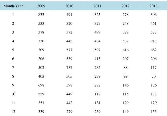
The data from Table 1consists of 60 monthly Malaria cases from January 2009 to December 2013 for age 1 to under 5 years. 2014 data set was not ready at the time of collection. This study assumes that the reporting and registering of monthly malaria cases remain the same throughout the study period. Since the study was done by collecting data from a single centre, it is difficult to generalize the results in the actual population.
4. Model-Building Process
The first step in this time series analysis is to plot the observations against time. Graphs from these observations are called time plot and they show up important features of the series such as trend, seasonality, outliers and discontinuities. The input data must be adjusted to form a stationary series, one whose values vary more or less uniformly about a fixed level over time. Trends can be adjusted by “regular differencing”, a process of compu-ting the difference between every two successive values, compucompu-ting a differenced series which has overall trend behavior removed. If a single differencing does not achieve stationarity, it may be repeated although rare to have more than two regular differencing’s. Where irregularities in the differenced series continue to be displayed, log or inverse functions can be specified to stabilize the series such that the remaining residual plot displays values approaching zero and without any pattern. This is the error term, equivalent to pure, white noise [11].
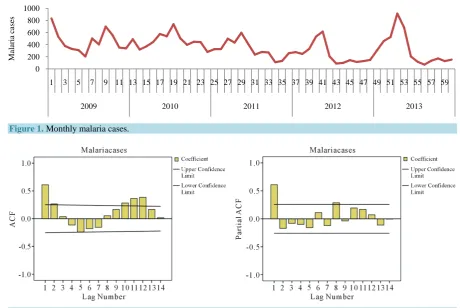
A visual inspection of the time series plot in Figure 1 suggests a stationary process with constant mean and variance.
4.1. Model Selection
Two graphical devices which are the autocorrelation function (ACF) and partial autocorrelation function (PACF) are used as guides to choosing one or more Autoregressive Integrated Moving Average (ARIMA) models that are appropriate.
Figure 2 describe the features of the data that is the autocorrelation plot and the partial autocorrelation plot. The ACF and PACF show that the ACF decays exponentially and the PACF has a single spike at lag 1 indicat-ing that the series is generated by an ARIMA (1, 0, 0) process,
(
1)
.t t t
[image:4.595.145.482.473.707.2]X = +µ φ X− −µ +e (2)
Table 1. 60 monthly Malaria cases from January 2009 to December 2013.
Month/Year 2009 2010 2011 2012 2013
1 833 491 325 278 306
2 533 320 327 248 461
3 378 372 499 329 527
4 330 445 434 532 913
5 309 577 597 616 682
6 206 539 415 207 206
7 502 737 235 88 117
8 403 505 279 99 70
9 698 398 272 146 136
10 559 449 112 115 173
11 351 442 131 129 129
12 339 279 259 149 153
Figure 1. Monthly malaria cases.
Figure 2.ACF and PACF of the monthly malaria cases.
4.2. Parameter Estimation
Equation (2) can now be used to estimate the parameter by least squares estimation. Reference [12] argue that because the method of moments is unsatisfactory for many models, we will consider the method of least squares estimation for our model. Given that our identified model is Xt= +µ φ
(
Xt−1−µ)
+et.We view this as a regression model with predictor variable Xt then apply the Least Squares estimation
proceeds by minimizing the sum of the differences. The estimators are µˆ and ˆφ can be obtained as follows:
1 ˆ n t t X n X
µ= =
∑
= (3)(
)(
)
(
)
60 1 2 60 2 1 2ˆ t t t .
t t
X X
X X
X X
φ = −
− = − − = −
∑
∑
(4)Calculations in Excel show that: ˆµ=X =361.48 and ˆφ=0.68. Hence, the model is
(
1)
361.48 0.68 361.48 .
t t t
X = + X− − +e (5)
4.3. Diagnostic Checks
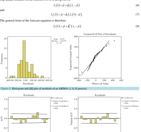
Verification of goodness of fit of any model should include a test as to whether the residuals form a white noise process. A portfolio of tests for goodness of fit of our model has been done in this paper.
The histogram shows that the average of residuals is approximately 0. The QQ plots are an effective tool for assessing normality. The QQ plot of residual observations in Figure 3 suggests that the points follow the straight line (45 degree line) closely implying that the residuals are normally distributed.
0 200 400 600 800 1000
1 3 5 7 9 11 13 15 17 19 21 23 25 27 29 31 33 35 37 39 41 43 45 47 49 51 53 55 57 59
2009 2010 2011 2012 2013
M
al
ar
ia cas
The autocorrelation plot show (see Figure 4) that only one value is outside the confidence limit which would not be regarded as significant on its own, three such values might be considered to be significant. All the terms of the partial autocorrelation plot are interior to the confidence limit suggesting that the residuals are a white noise.
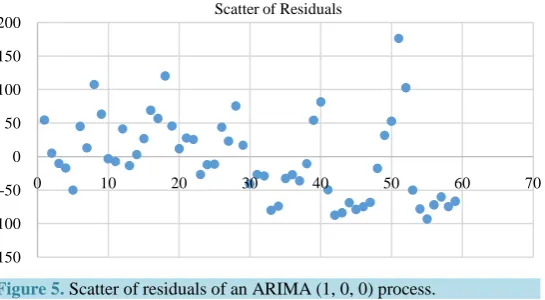
Our other diagnostic check is to inspect a scatter plot of the residuals over time in Figure 5. The model is adequate, since the residual scatter plot show a rectangular scatter around a zero horizontal level with no trends present.
5. Forecasting
Box-Jenkins approach to forecasting stationary time series is relatively simple. The forecast value of Xt k+ given all observations up until n the k-step ahead forecast is denoted by x kˆt
( )
. The one-step ahead and two- step ahead forecasts for an ARIMA (1, 0, 0) are given by:( )
ˆ1(
)
ˆt 1 ˆ ˆt ˆ
x = +
µ φ
x −µ
(6) and( )
ˆ1(
( )
)
ˆt 2 ˆ ˆt 1 ˆ .
x = +µ φ x −µ (7)
The general form of the forecast equation is therefore
( )
ˆ1(
)
ˆ ˆ k ˆ
t t
[image:6.595.87.544.231.659.2]x k = +
µ φ
x −µ
(8) [image:6.595.91.539.534.706.2]Figure 3. Histogram and QQ plot of residuals of an ARIMA (1, 0, 0) process.
Figure 5. Scatter of residuals of an ARIMA (1, 0, 0) process.
for k≥1. We want to forecast with µ =ˆ 361.48 and ˆφ=0.68 considering the data in Table 1.
( )
(
)
60 1 361.48 0.68 153 361.48 219.714
x = + − =
( )
(
) (
2)
60 2 361.48 0.68 153 361.48 265.079
x = + − = .
6. Discussion
ARIMA (1, 0, 0) model developed in this paper attempts to provide the best possible model for predicting mala-ria cases per month in the future based on observed malamala-ria cases over the years. The results also indicate that the malaria cases will continue to occur in the near future if appropriate intervention measures are not initiated on time. The potential implication of this study is that by developing forecasting models for predicting the ex-pected number of malaria cases in advance, timely prevention and control measures can be effectively planned like eliminating vector breeding places, spraying insecticides, and creating public awareness. The study also provides a model to foresee and allocate appropriate resources to maintain a steady decrease and combat malaria. The ARIMA model used in this paper can also be applied to other diseases like Ebola. These results can also be used to sensitize travelers about malaria risk to take necessary precautionary measures.
7. Conclusion
In this paper, the Box-Jenkins modelling procedure is discussed to determine an ARIMA model and go further to forecasting. We considered data of Malaria cases from Ministry of Health (Kabwe District)-Zambia for the period, 2009 to 2013 for age 1 to under 5 years. Results show that an appropriate model is simply an ARIMA (1, 0, 0) due to the fact that, the ACF decays exponentially and the PACF has a spike at lag 1 which is an indication of the said model. The forecasted Malaria cases for January and February, 2014 are 220 and 265, respectively. Finally, the study can be done on a wider area of Zambia and further research can be done to evaluate the effec-tiveness of integrating the forecasting model into the existing disease control program in terms of its impact in reducing the disease occurrence. These will be studied elsewhere.
Acknowledgements
The authors are thankful to the Ministry of Health for providing the data. Department of Mathematics and Sta-tistics, Mulungushi University for using their resources and to all the people who helped in making comments on this paper.
References
[1] Abebe, A., Dagnachew, M., Mikrie, M., Meaza, A. and Melkamu, G. (2012) Ten Year Trend Analysis of Malaria Pre-valence in Kola Diba, North Gondar, Northwest Ethiopia. Parasites and Vectors, 5, 173.
http://dx.doi.org/10.1186/1756-3305-5-173
[2] World Health Organization (2011) World Malaria Report. Geneva, Switzerland. -150
-100 -50 0 50 100 150 200
0 10 20 30 40 50 60 70
www.who.int/malaria/world_malaria_report_2011
[3] Box, G.E. and Jenkins, G.M. (1994) Time Series Analysis: Forecasting and Control. Prentice Hall, Englewood Cliffs. [4] Pankratz, A. (1983) Forecasting with Univariate Box-Jenkins Models. Wiley & Sons, Inc., New York.
http://dx.doi.org/10.1002/9780470316566
[5] Levenback, H. and Cleary, J.P. (2006) Forecasting Practice and Process for Demand Management. Thomson Brooks/ Cole, Belmont.
[6] Tarekegn, A.A., Sake, J.D., Gerard, B., Awash, T., Asnakew, K., Dereje, O., Gerrit, J. and Habbema, J.D.F. (2002) Forecasting Malaria Incidence from Historical Morbidity Patterns in Epidemic-Prone Areas of Ethiopia: A Simple Seasonal Adjustment Method Performs Best. Tropical Medicine and International Health, 7, 851-857.
http://dx.doi.org/10.1046/j.1365-3156.2002.00924.x
[7] Ekezie, D.D., Opara, J. and Okenwe, I. (2014) Modelling and Forecasting Malaria Mortality Rate Using SARIMA Models (A Case Study of Aboh Mbaise General Hospital, Imo State Nigeria). Science Journal of Applied Mathematics
and Statistics, 2, 31-41. http://dx.doi.org/10.11648/j.sjams.20140201.15
[8] Adebola, P.A. and Okereke, R.W. (2007) Increasing Burden of Childwood Severe Malaria in a Nigeria Tertiary Hos-pital from 2000 to 2005. An Unpublished Research Work.
[9] Varun, K., Abha, M., Sanjeet, P., Geeta, Y., Richa, T., Deepak, R. and Saudan, S. (2014) Forecasting Malaria Cases Using Climatic Factors in Delhi, India: A Time Series Analysis. Hindawi Publishing Corporation Malaria Research
and Treatment, 2014, Article ID: 482851.
[10] Dobre, I. and Alexandru, A. (2008) Modelling Unemployment Rate Using Box-Jenkins Procedure. Journal of Applied
Quantitative Methods, 3.
[11] Wei, W. (1990) A Time Series Analysis: Univariate and Multivariate Methods. Addison-Wesley Publishing Company, Inc., New York.
[12] Cryer, J.D. and Chan, K.S. (2008) Time Series Analysis with Application in R. Springer, New York.