GMM Estimation of short dynamic panel data models with error cross sectional dependence

Munich Personal RePEc Archive

GMM Estimation of short dynamic panel

data models with error cross-sectional

dependence

Sarafidis, Vasilis

University of Sydney, Monash University

January 2009

GMM Estimation of Short Dynamic Panel Data Models With

Error Cross-Sectional Dependence

Vasilis Sara…disy

This version: December 2011

Abstract

This paper considers estimation of short dynamic panel data models with error cross-sectional dependence. It is shown that under spatially correlated errors, an additional, generally non-redundant, set of moment conditions becomes available for each i speci…cally, instruments with respect to the individual(s) which unitiis spatially correlated with. We demonstrate that these moment conditions remain valid when the error term contains a common factor component, in which situation the standard moment conditions with respect to individualiitself are invalid-ated, and thereby the standard dynamic panel GMM estimators are inconsistent. The resulting estimators are computationally attractive and do not require estimating the number of unob-served factors. Simulated experiments show that the resulting method of moments estimators perform well in terms of both median bias and root median square error.

Key Words: Dynamic Panel Data, Spatial Dependence, Factor Structure Dependence, Generalised Method of Moments.

JEL Classi…cation: C13; C15; C33.

1

Introduction

In developing the theory of GMM estimation of short dynamic panel data models, it is commonly assumed that the residuals are independently distributed across individuals (see e.g. Anderson and Hsiao, 1981, pg. 598, Arellano and Bond, 1991, pg. 278, Arellano, 1993, pg. 88, Ahn and Schmidt, 1995, pg. 7, Blundell and Bond, 1998, page 118, and others). This assumption is usually made for identi…cation purposes rather than descriptive accuracy with the hope, presumably, that by conditioning on a su¢cient number of explanatory variables, what is left over can be treated as a purely idiosyncratic disturbance that is uncorrelated in the cross-sectional dimension. On the other hand, this rather strong assumption is somewhat relaxed in empirical applications involving dynamic panels by allowing for common variations in the dependent variable at any given point in time using a two-way error components disturbance (e.g. Arellano and Bond, 1991, pg. 288, Blundell and Bond, 1998, pg. 137, Bover and Watson, 2005, pg. 1975). In practice, however, this formulation is unlikely to be adequate to remove all correlated behaviour in the residuals and this may invalidate the point estimates of the parameters, as well as inferences; see e.g. Sara…dis and Robertson (2009).

Error cross-sectional dependence may arise for various reasons in practice; for example, it may be due to the presence of spatial correlations speci…ed on the basis of economic and social distance (Conley, 1999) or relative location (Anselin, 1988), as well as due to the presence of unobserved components that give rise to a common factor speci…cation in the disturbances with a …xed number

I would like to thank Takashi Yamagata and Neville Weber for helpful comments and suggestions.

y_{Discipline of Operations Management and Econometrics, University of Sydney, and Department of Econometrics}

of factors (e.g. Goldberger, 1972, and Jöreskog and Goldberger, 1975). Methods that account for spatial dependence in panel data models have been proposed by Mutl (2006), Kapoor, Kelejian and Prucha (2007), Lee and Yu (2010) among others. Methods that deal with a multi-factor error structure have been proposed by Robertson and Symons (2007), Phillips and Sul (2003), Moon and Perron (2004), Bai (2006), Pesaran (2006), Sara…dis and Yamagata (2010) among others. These methods are theoretically justi…ed in panels where the number of time series observations (T) is large and/or (some of) the covariates are strictly exogenous with respect to the purely idiosyncratic disturbance. Valid methods for …xed T and weakly exogenous, or endogenous regressors have been proposed by Ahn, Lee and Schmidt (2006), Bai (2010), Robertson, Sara…dis and Symons (2010). These methods are non-linear and require estimating the number of unobserved factors as well as the factors themselves. An overview of recent developments in the literature is provided by Sara…dis and Wansbeek (2012).

The present paper investigates the e¤ect of spatial dependence in dynamic panel data models. It is shown that an additional set of moment conditions becomes available in particular, instruments with respect to the individual(s) which unitiis spatially correlated with. In many practical circum-stances these moment conditions are not redundant in the sense that the asymptotic variance of the GMM estimator from the enlarged set of moment conditions is smaller than the GMM estimator that uses the smaller set of moment conditions, i.e. those instruments with respect to individual i

only. We develop two GMM estimators. One is based on …rst-di¤erenced equations and is similar to the Arellano and Bond (1991) GMM estimator. The other one combines equations in …rst-di¤erences and in levels, yielding a system GMM estimator. Unlike the standard system GMM, however, this estimator remains consistent even if the process is not mean-stationary. This is important because mean-stationarity cannot be theoretically founded in a large number of applications.

Most notably, it is demonstrated that the spatial moment conditions remain valid even when the error term contains a common factor component, in which case the standard moment conditions with respect to lagged values of the endogenous regressor are invalidated. The resulting estimators are computationally attractive since the moment conditions are linear in the parameters, and they do not require estimating the number of unobserved factors or the factors themselves (assuming that theory suggests a particular number of factors to exist) for consistent estimation of the structural parameters. In addition, the set of regressors can be strictly exogenous, or endogenous, while T

can be either …xed or large, provided that the number of moment conditions utilised does not grow with T. The main requirement is the speci…cation of a spatial weighting matrix, which is common practice in the spatial literature.

The structure of the paper is as follows. The following section speci…es the panel regression model, discusses the basic assumptions employed and derives the consistency and asymptotic normal-ity of the standard …rst-di¤erenced and system GMM estimators under spatial dependence. Section 3 analyses the properties of the spatial instruments that become available. Section 4 demonstrates that these instruments remain valid even if the error contains a common factor component. The performance of the resulting estimators is investigated in Section 5 using simulated data. A …nal section concludes.

2

Model Speci…cation and Standard Moment Conditions

This section investigates the e¤ect of spatial dependence on dynamic panel data estimation. Without loss of generality and for easy of exposition we will consider the following panel AR(1) model:

yit = yit 1+uit, j j<1,i= 1; :::; N,t= 1; :::; T,

uit = i+"it,"it = N

X

j=1

where the initial observation is given by

yi0 = 0 i+ 1"i0,"i0 =

N

X

j=1

wij;N j0+ i0. (1)

For 0 = 1=(1 ) the process is mean-stationary, and if, in addition, 1 =

p

1=(1 2_{) the}

process is covariance-stationary. We do not necessarily want to impose these restrictions at this stage.

Stacking the model overiyields

yt= yt 1+ut= yt 1+ +"t= yt 1+ +PN t, (2)

where yt = (y1t; :::; yN t)0, yt 1 = (y1t 1; :::; yN t 1)0, ut = (u1t; :::; uN t)0, = ( 1; :::; N)0, "t =

("1t; :::; "N t)0, t= ( 1t; :::; N t)0,WN is anN N matrix andPN =IN + WN. ytcan be written

as

yt= ty0+

1 t

1 +PN

t 1

X

=0

t , (3)

and from (1) we have y0 = 0 + 1PN 0 . Therefore, yt can be expressed as a linear form of the

innovations, and ,

yt N 1

= ( _t PN)

N N(T+1)N(T+1) 1

+ _0;t ,

N 1

(4)

where, following a similar approach to Mutl (2006), _t= 1 t; t 1; :::; 0;01 T t is a1 (T + 1)

row vector, = ( 0

0; :::; 0T)

0

is aN(T + 1) 1 column vector that contains all the elements of the purely idiosyncratic error component, while _0;t = h₁1 + t 0 ₁1

i

. Observe that "t can

also be expressed as a linear form of as follows:

"t N 1

= (dt PN)

N N(T+1)N(T+1) 1

, (5)

wheredt is a1 (T + 1)row vector and consists of the(t 1)th row of(0T 1 1; D), whileDis the

(T 1) T matrix …rst-di¤erence operator (see e.g. Arellano, 2003, pg. 15) de…ned as

D

2 6 6 6 4

1 1 0 0 0 0 1 1 0 0

..

. . ..

0 0 0 1 1

3 7 7 7 5.

Similarly, ut can be expressed as

ut N 1=

e0_t+1 PN

N N(T+1) N(T+1) 1

+ ,

N 1

(6)

where et+1 denotes the elementary(T+ 1) 1 vector with1 in the(t+ 1)th position.

Taking …rst-di¤erences in(2)yields

yt= yt 1+ "t= yt 1+PN t,t= 2; :::; T. (7)

One can express yt as a linear form of the innovations as follows:

yt N 1

= ( _t PN)

N N(T+1)N(T+1) 1

+ _0;t ,

N 1

with _{t 1} = 1( 1) t 2;( 1) t 3; :::;( 1) 0;1;01 T (t 1) is a 1 (T + 1) row vector, 0;t 1 = t 2 0(1 ) t 2 , while , have been de…ned above. Stacking (2) and (7) over

t= 2; :::; T yields

y

N(T 1) 1

= y 1

N(T 1) 1

+ u,

N(T 1) 1

(9)

and

y

N(T 1) 1

= y 1

N(T 1) 1

+ ",

N(T 1) 1

(10)

respectively, where y= (y0

2; :::;y0T)

0

,y 1 = y01; :::;y0T 1

0

,u= (u0

2; :::;u0T)

0

, y= ( y0

2; :::; y0T)

0

, y 1= y01; :::; y0T 1

0

, "= ( "0₂; :::; "0_T)0.

LetZD =diag Y0; Y1; :::; YT 2 be a N(T 1) T(T 1)=2 block-diagonal matrix, where a

typical block is Ys _{= (y}

0;y1;; :::;ys), aN (s+ 1) matrix, where y = (y1 ; y2 ; :::; yN )0, aN 1

vector. Also, let ZL = diag( y1; y2; :::; yT 1) be a N(T 1) (T 1) matrix, where each

block is given by ys = ( y1s; y2s; :::; yN s)0, a N 1 vector. The following assumptions are

maintained:

Assumption 1 (error components): (i) The random variables _f it: 1 i N,0 t Tg are

independently distributed with zero mean and …nite variance 2_{. Furthermore,sup}

1 i N;0 t T

E_j itj4+ <1for some >0. (ii) The random variables f i: 1 i Ng are independently

distributed with zero mean and …nite variance 2_{. Furthermore, sup}

1 i NEj ij4+ <1 for

some >0. (iii) The processes_f itg and f igare totally independent.

Assumption 2 (weighting matrix and space of MA parameter): (i) All diagonal elements of WN equal zero. (ii) The spatial moving average parameter satis…es 2 ( c1; ; c2; ) with

0 < c1; ; c2; c < 1. (iii) The matrix WN is non-singular and PN = IN + WN is

non-singular for all ₂ ( c1; ; c2; ). (iv) The row and column sums of WN and (IN+ WN) are

bounded uniformly in absolute value.

The assumptions above are standard in the spatial literature, see e.g. Kelejian and Prucha (2010). Notice that Assumption 1 permits cross-sectional heteroskedasticity in "it, through the weighting

matrix WN. Serial independence in the error can be relaxed by allowing "it to follow a …nite MA

process. An AR process can be accommodated using further lags of y on the right-hand side of the model. Assumption 2(i) is just a normalisation of the model and implies that no individual is viewed as its own neighbour. Assumptions 2(ii)-(iiii) concern the parameter space of and are discussed in detail by Kelejian and Prucha (2010, Section 2.2). Assumption 2(iv) implies that there is no dominant unit in the sample, i.e. an individual unit that is correlated with all remaining individuals. We will study the factor structure case, which violates this scenario, in Section 4. Notice that the assumptions above do not depend on a particular ordering of the data, which can be arbitrary. For reasons of generality the elements of WN, and by implication of y with a slight

abuse of notation, are permitted to depend on N, that is to form triangular arrays. This is due to the fact that for “boundary” elements the connectedness structure may change as new data points are added. This implies that the asymptotics require the use of a CLT for triangular arrays (see e.g. Davidson, 1994, Ch. 24).

The following proposition shows that the following moment conditions remain valid for the panel autoregressive model with spatially correlated errors.

Proposition 1 Under Assumptions 1-2, the followingT(T 1)=2 moment conditions are valid in the …rst-di¤erenced model (10):

mN;D( ) =N 1ZD0 " p

!0. (11)

Furthermore, under mean-stationarity, 0 = 1=(1 ), the following T 1 moment conditions are

valid in the levels model (9):

mN;L( ) =N 1ZL0u p

Proof. See Appendix A.

The above proposition demonstrates that instruments with respect to lagged values of the en-dogenous regressor remain valid under spatial dependence. Therefore, under certain regularity conditions it will be shown that Generalised Method of Moment estimators making use of these moment conditions are consistent and asymptotically normal with mean zero. In particular, de…ne

ZS Z₀D _Z0

L ;yS

y

y ;y 1;S

y 1

y 1 ;uS

"

u .

Also, letA1;D;N andA1;S;N be sequences of possibly random, non-negative de…nite matrices of order

1;D 1;D and 1;S 1;S, respectively, where 1;D=T(T 1)=2and 1;S =T(T 1)=2 +T 1.

The following assumption is employed for the identi…cation of the autoregressive parameter, .

Assumption 3(i) (identi…cation of ): N 1Z0

DZD p

!QZD,N

1_Z0

D y 1 p

!qZD y 1,N

1_Z0

SZS p

!QZS,N

1_Z0

Sy 1;S p

!qZSy 1;S, all …nite matrices (vectors) with full column rank (non-zero

entries). A1;D;N and A1;S;N have full rank and A1;D;N p

!A1;D,A1;S;N p

!A1;S.

The …rst-di¤erenced (FD) GMM estimator is de…ned as the minimiser of the following quadratic form:

bD(A1;D;N) arg minmN;D( ) 0_A

1;D;NmN;D( ). (13)

Combining(11) and (12)yields

mN;S( ) =N 1ZS0uS p

!0. (14)

The system (SYS) GMM estimator is de…ned as the minimiser of the following quadratic form:

bS(A1;S;N) arg minmN;S( )A1;S;NmN;S( ), (15)

Setting the …rst-order conditions equal to zero and solving for the unknown value of in(13) and

(15) yields

bD = y0 1ZDA1;D;NZD0 y 1 1 y0 1ZDA1;D;NZD0 y , (16)

and

bS = y0 1;SZSA1;S;NZS0y 1;S 1 y0 1;SZSA1;S;NZS0yS , (17)

respectively. The following theorem establishes the consistency and asymptotic normality of the above estimators.

Theorem 2 Suppose Assumptions 1-3(i), and(11) hold true. Let 1;D;N =var

h_p

NmN;D( )

i be a sequence of symmetric, non-negative de…nite matrices with rank greater than or equal to _1;D, such that min( 1;D;N) c >0, and 1;D;N

p

! 1;D =asy:var

h_p

NmN;D( )

i

. The GMM estimator in

(16) is consistent and

p

N _bD(A1

;D;N)

d

!N(0; VD), (18)

where

VD =

h

qZD y 1A

0

1;Dq0ZD y 1

i 1

qZD y 1A1;D 1;DA1;Dq

0

ZD y 1

h

qZD y 1A1;Dq

0

ZD y 1

i 1

. (19)

In addition to the assumptions above, suppose that(12)holds true and let 1;S;N =var

h_p

NmN;S( )

i

be a sequence of symmetric, non-negative de…nite matrices with rank greater than or equal to _1;S, such that min( 1;S;N) c >0, and 1;S;N !p 1;S =asy:var

h_p

NmN;S( )

i

. The GMM estimator in (17) is consistent and

p

where

VS =

h

qZSy 1;SA1;Sq 0

ZSy 1;S

i 1

qZSy 1;SA1;S 1;SA1;Sq 0

ZSy 1;S

h

qZSy 1;SA1;Sq 0

ZSy 1;S

i 1

. (21)

Proof. See Appendix A.

A …rst-stage choice forA1;D;N can be such that

A1;D =N 1ZD0 DD0 IN ZD,

which takes into account that the …rst-di¤erenced operator creates serial correlation in the errors but ignores spatial correlation. Similarly, for A1;S;N one can choose

A1;S =N 1ZS0

(D IN) (D IN)0 0

0 (IT 1 IN) ZS.

The optimal GMM estimators are obtained by replacingA1;D;N andA1;S;N by 1;D;N1 and 1;S;N1 ,

respectively, in which case (19) and (21)reduce to

VD =

h

qZD y 1

1

1Dq0ZD y 1

i 1

,

and

VS =

h

qZSy 1;S

1 1;Sq

0

ZSy 1;S

i 1

.

The distributional results hold as well if the unobserved _1;D;N1 , _1;S;N1 are replaced by consistent estimates. In particular, notice that 1;D;N can be partitioned as follows:

1;D;N =

2 6 4

1;22;D;N 1;2T;D;N

. ..

1;T2;D;N 1;T T;D;N

3 7 5,

where 1;ts;D;N = N 1EYt 20 "t "0sYs 2. Letting the pqth element of 1;ts;D;N be denoted by

!1;pq;ts;D;N, we have

!1;pq;ts;D;N = N 1Ey0p "t "0syq

= N 1 0 0_pdt PN0 PN + 0;p 0(dt PN)

0 _d0

s q PN0 PN + 0;q 0(ds PN)

= N 12tr 0_pdt PN0 PN d0s q PN0 PN

+ _{0;p 0;q}tr[(dt PN) (ds PN) ],

where = 2_I

N(T+1), = 2IN and the remaining variables have been already de…ned.1

There-fore, an expectations based operator for !1;pq;ts;D;N will replace the true value of the parameters

above by their consistent estimates, obtained from the …rst stage. A consistent estimate for , required to compute PN, can be obtained based on the estimator proposed by Fingleton (2008),

applied on the residual vector bu=y by 1; see also Kapoor, Kelejian and Prucha (2007).

An alternative estimator for 1;ts;D;N can be obtained by ignoring the fact that the instruments

are stochastic variables, based on

e_1;D;N =N 1Z_D0 b ";NZD,

1_{This expression easily follows from the expectation of} 2

3;ts;N in the proof of Proposition 3 in the Appendix with

f

where b ";N is a consistent estimate of

E " "0 =E (D PN) 0 D0 PN0 = 2(D PN) D0 PN0 ,

with unknown parameters 2 _{and . This is sub-optimal in the sense that e}

1;D;N is not a

consist-ent estimator for 1;D;N, however, it is computationally simpler and results in a consistent GMM

estimator of . Similar analysis applies to 1;S;N. Block bootstrapping procedures for spatially

dependent observations are also available; see e.g. Hall (1985) and Anselin (1990). We will explore this alternative in Section 3.1.

3

Spatial Instruments: Validity, Relevance and Redundancy

It turns out that under spatially correlated errors, an additional set of moment conditions becomes valid and is relevant in the sense that it is correlated with the endogenous regressor. This is demonstrated in the proposition below. In particular, let ZeD =diag WfNY0;WfNY1; :::;WfNYT 2

be aN(T 1) T(T 1)=2block-diagonal matrix, wherefWN =WN+WN0 is a symmetric matrix,

and Ys _{has been de…ned above. E¤ectivelyWf}

N is a matrix theith row of which contains non-zero

values at the entries corresponding to the individuals which unit iis spatially correlated with. Also, let ZeL =diag fWN y1;WfN y2; :::;fWN yT 1 be aN(T 1) (T 1) matrix, where ys has

been de…ned previously.

Proposition 3 Under Assumptions 1-2, the followingT(T 1)=2 moment conditions are valid in the …rst-di¤erenced model (10):

e

mN;D( ) =N 1ZeD0 " p

!0, (22)

with

e

gN;D( ) =N 1ZeD0 y 1

p

!q_Ze

D y 1, (23)

where q_Ze

D y 1 = q1;D; :::; qT(T 1)=2;D

0

denotes a T(T 1)=2 1 column vector with qk;D6= 0, in

general. Furthermore, the following T 1 moment conditions are valid in the levels model (9): e

mN;L( ) =N 1ZeL0 u p

!0, (24)

with

e

gN;L( ) =N 1ZeL0y 1

p

!q_Ze

Ly 1, (25)

where q_Ze

Ly 1 = (q1;L; :::; qT 1;L)

0

denotes a (T 1) 1 column vector with qk;L6= 0, in general.

Proof. See Appendix A.

The above proposition shows that the spatial instruments are valid and relevant as well, so long as ₆= 0, as shown in the appendix.

Remark 4 Observe that unlike Proposition 1 we have not imposed mean stationarity for the equa-tions in levels. Intuitively, this is because E _{i j} = 0 ₈i ₆= j, under the maintained assumptions. Therefore, the spatial moment conditions in the equations in levels are valid in this case even if the standard moment conditions are not. We will investigate the consequences of this result in simulations.

De…ne

Z_De

N(T 1) T(T 1)

h

ZD ; ZeD

i

; Z_Le

N(T 1) 2(T 1)

h

ZL ; ZeL

i

; Z_Se

N(T 1) [T(T 1)+2(T 1)]

m_N;De( ) N 1Z0_e

D ",

and

m_N;Se( ) N 1Z0_e

S uS:

Let A2;D;N and A2;S;N be sequences of possibly random, non-negative de…nite matrices of order

2;D 2;D, and 2;S 2;S, respectively, where 2;D = T(T 1), 2;S = T(T 1) + 2 (T 1).

Furthermore, let qZ_De y 1 = q

0

ZD y 1;q

0 e

ZD y 1

0

, qZ_Sey 1;S = q 0

Z_De y 1;q

0

Z_Ley 1

0

with qZ_Ley 1 =

q0

ZLy 1;q

0 e

ZLy 1

0

. The following assumption is employed for the identi…cation of :

Assumption 3(ii) (identi…cation of ):N 1_Z0 e

DZDe p

!QZ_De,N 1Z_D0_e y 1

p

!qZ_De y 1,N

1_Z0 e

SZSe p

!QZ_Se, ,N 1Z_S0_ey 1;S p

!qZ_Sey 1;S, all …nite matrices (vectors) with full column rank (non-zero

entries). A2;D;N and A2;S;N have full rank, such thatA2;D;N p

!A2;D,A2;S;N p

!A2;S.

Let

eD(A2;D;N) =

h

y0 ₁Z_DeA2;D;NZ_D0_e y 1

i 1h

y0 ₁Z_DeA2;D;NZ_D0_e y

i

, (26)

and

eS(A2;S;N) =

h

y0 _1;SZ_SeA2;S;NZ_S0_ey 1;S

i 1h

y0 _1;SZ_SeA2;S;NZ_S0_eyS

i

, (27)

be the FD and SYS GMM estimators that combine the standard and spatial instruments. The following theorem establishes the consistency and asymptotic normality of these estimators.

Theorem 5 Suppose Assumptions 1-3(ii), and(22),(23)hold true. Let 2;D;N =var

h_p

Nm_N;De( )i

be a sequence of symmetric non-negative de…nite matrices with rank greater than or equal to _2;D, such that min( 2;D;N) c >0, and 2;D;N !p 2;D =asy:var

h_p

Nm_N;De( )i. The GMM estim-ator in (26) is consistent and

p

N(eD )!d N 0; VDe , (28)

where

V_De =hqZ_De y 1A2;Dq

0

Z_De y 1

i 1

qZ_De y 1A2;D 2;DA2;Dq

0

Z_De y 1

h

qZ_De y 1A2;Dq

0

Z_De y 1

i 1

.

In addition to the assumptions above, suppose that (12), (24)-(25) hold true and let 2;S;N =

varhpNm_N;Se( )i be a sequence of symmetric, non-negative de…nite matrices with rank greater than or equal to _2;S, such that min( 2;S;N) c >0, and 2;S;N !p 2;S =asy:var

h_p

Nm_N;Se( )i. The GMM estimator in (27) is consistent and

p

N(_eS )!d N 0; VSe , (29)

where

V_Se=hqZ_Sey 1;SA2;Sq 0

Z_Sey 1;S

i 1

qZ_Sey 1;SA2;S 2;SA2;Sq 0

Z_Sey 1;S

h

qZ_Sey 1;SA2;Sq 0

Z_Sey 1;S

i 1

.

Proof. See Appendix A.

of the GMM estimator, the additional instruments are redundant.2 _{To shed some light on this issue}

we will consider the case where T = 2 for the model in …rst-di¤erences; there is a single equation given by

yi2= yi1+ "i2,

and a single instrument with respect to lagged values of the endogenous regressor of individual i, such that the reduced form (instrumental variable regression) equation is

yi1 = yi0+ei.

The FD GMM estimator of reduces to a simple IV estimator, given by

b = covc ( yi2;byi0)

c var(byi0)

= covc [ ( yi1+ "i2);byi0]

c var(byi0)

= covc [ (byi0+ei) + "i2;byi0]

c var(_byi0)

= +covc ( "i2; yi0)

b cvar(yi0)

,

where the last equality holds becauseei is orthogonal to yi0 by construction. Hence, we have p

N(_b ) =pNcovc ( "i2; yi0)

b cvar(yi0)

= 1

b cvar(yi0)

N

X

i=1

"i2yi0= p

N. (30)

Using Proposition 1 and Theorem 2 we have

1

b cvar(yi0)

p

! _var1_(y

i0)

, (31)

while _P

N

i=1 "i2yi0 p

N

d

!N[0;var( "i2)var(yi0)], (32)

since

var PN

i=1_p "i2yi0

N ! = 1 Nvar N X i=1

"i2yi0

!

=E "2_i2 E y2_i0 . (33)

A direct application of Slutsky theorem yields

p

N(b )_!d N(0; V_b), (34)

where

V_b= var₂ ( "i2)

var(yi0)

. (35)

In addition, there exist spatial instruments with respect to the individual(s) unit i is spatially correlated with. The instrumental variable equation for the two-stage least-squares (2SLS) estimator that uses the enlarged set of moment conditions is

yi1= 1yi0+ 2

N

X

j=1

wijyj0+wi.

The 2SLS estimator of is given by

e =

c cov

2

4 yi2;b1yi0+b2

N

X

j=1

wijyj0

3 5

c var

2

4b1yi0+b2

N

X

j=1

wijyj0

3 5 = + c cov 0

@ "i2;b1yi0+b2

N

X

j=1

wijyj0

1 A

c var

0

@b1yi0+b2

N

X

j=1

wijyj0

1 A

, (36)

where, similarly as above, wi is orthogonal to yi0 and

N

X

j=1

wijyj0 by construction.3 Therefore, one

has

1

c var

2

4b1yi0+b2

N

X

j=1

wijyj0

3 5 p ! 1 var 2

4 ₁yi0+ 2

N

X

j=1

wijyj0

3 5

, (37)

and

PN i=1 "i2

2

4b1yi0+b2

N

X

j=1

wijyj0

3 5 p N a N 2

40;var( "i2) var

0

@ ₁yi0+ 2

N

X

j=1

wijyj0

1 A 3 5.

The asymptotic distribution of pN(_e )is

p

N(_e )_!d N(0; V_e), (38)

where

V_e = var( "i2)

var 0

@ ₁yi0+ 2

N

X

j=1

wijyj0

1 A

= var( "i2)

2

1var(yi0) + 22var

0 @

N

X

j=1

wijyj0

1

A+ 2 _{1 2}cov 0 @yi0;

N

X

j=1

wijyj0

1 A

. (39)

It is straightforward to show that the denominator in (39) is larger than in (35) and therefore _e is asymptotically more e¢cient than b. This holds true unless ₂ = 0, in which case ₁ = and e is asymptotically equivalent to _b. This is an intuitive result because ₂ = 0implies that, conditional on yi0,

N

X

j=1

wijyj0 is not correlated with the endogenous regressor. We will investigate further the

condition ₂ = 0 by considering the …rst-stage coe¢cient _b2, which equals

b2 =

c cov

0 @ yi1;

N

X

j=1

wijyj0

1

A cvar(yi0) covc ( yi1; yi0)covc

0 @yi0;

N

X

j=1

wijyj0

1 A

c

var(yi0)varc

0 @

N

X

j=1

wijyj0

1 A cov_c

0 @yi0;

N

X

j=1

wijyj0

1 A

2

p

! 2=

cov 0 @ yi1;

N

X

j=1

wijyj0

1

Avar(yi0) cov( yi1; yi0)cov

0 @yi0;

N

X

j=1

wijyj0

1 A

var(yi0)var

0 @

N

X

j=1

wijyj0

1 A cov

0 @yi0;

N

X

j=1

wijyj0

1 A

2 . (40)

3_{Notice that it is also possible to investigate the properties of the GMM estimator that makes use of the optimal}

Without loss of generality suppose that the weighting matrix used is circular4_{, such that}

W=

2 6 6 6 6 6 6 4

0 1 0 : : : : : 0 0 0 1 0 : : : : 0

: : : : : : : : : : : : : : : : : :

0 : : : : 0 0 0 1 1 : : : : : 0 0 0

3 7 7 7 7 7 7 5

. (41)

One can show that

var(yi0) = 20 2+ 21 1 + 2 2;

var 0 @

N

X

j=1

wijyj0

1

A = 2 2₀ 2+ 2₁ 1 + 2 2 ;

cov( yi1; yi0) = ( 1) 0 2 0

1 1 +

2

1 2u 1 + 2 ;

cov 0 @ yi1;

N

X

j=1

wijyj0

1

A = 2 ( 1) 2₁ 2;

cov 0 @yi0;

N

X

j=1

wijyj0

1

A = 2 2₁ 2: (42)

As a result, we have

2=

2 ( 1) 2₁ 2h 2₀ 2+ 2₁ 1 + 2 2 [ 0 2 0 ₁1 + 21 1 + 2 2]

i

2h 2₀ 2₊ 2

1 1 + 2 2 2 2 21 2 2

i

=

( 1) 2₁ 2h 2

0 2 0 2 0 ₁1

i

2

0 2+ 21 1 + 2 2 2 2 21 2 2

= 0

2

1 2 2

4

0 4+ 2 20 21 2 1 + 2 2+ 41 1 + 4 4

. (43)

Therefore, we can see that ₂ = 0for either 0 = 0, or 1 = 0or = 0. The last two zero conditions

imply that the covariance between the endogenous regressor and the spatial instruments equals zero, as it is clear from (42). It is worth mentioning that ₂ does not depend on the value of so long as 0 and 1 are not a functions of . Furthermore, since the denominator in 2 is always a

non-negative number, ₂ 0for 0 and 0 0. The following …gure illustrates graphically the value

of ₂ for ₂ [0;1] and 0 2 [0;4], setting 21 = 2 = 2 = 1. Observe that for any 0 > 0, the

value of the function increases as approaches unity. On the other hand, for any given >0 the value of the function initially gets larger as 0 increases from zero to a positive value, although it

approaches zero as 0 increases further to large positive values. As an implication, if they process

is mean-stationary such that 0 = 1=(1 ), the spatial instruments become redundant as !1

regardless of the value of . Of course, at the same time instruments with respect to lagged values of the endogenous regressor for individual i become weak for _! 1. This in turn implies that the spatial instruments become weak as well, given redundancy. We will investigate further the properties of GMM estimators that make use of spatial instruments using simulated data in Section 3.1.

Figure 1

Another issue that arises is dominance; in particular, suppose that there is a dominant cross-sectional unit which is correlated with all remaining individuals. It turns out that instruments with respect to the dominant individual are always redundant. To see this, let the dominat unit be the

Nth individual. We have

plim_N!1N 1

N

X

i=1

yN s "it=yN splimN!1N 1

N

X

i=1

"it= 0, (44)

and

plim_N!1N 1

N

X

i=1

yN s yit 1 =yN splimN!1N 1

N

X

i=1

yit 1 = 0. (45)

Therefore, the instrument with respect to the dominant unit is uncorrelated with yit 1. Intuitively,

if the same variable is used as instrument for all individuals, then it is …xed in the cross-sectional dimension and therefore it is asymptotically uncorrelated with the endogenous regressor. Notice that the existence of a dominant unit violates the uniform boundedness condition of spatial dependence, and indeed one of the conditions in Theorem 1.

3.1 A Short Monte Carlo Investigation

We will investigate the …nite-sample performance of the estimators above using simulated data. The underlying generating process is given by

yit= yit 1+ i+"it,"it= N

X

j=1

wij;N jt+ it,i= 1; :::; N,t= 1; :::; T, (46)

where wij;N denotes the ijth element of WN, which is formulated as in (41), i i:i:d:N 0; 2 , it i:i:d:N 0; 2 . The initial value is

yi0 = 0 i+ 1"i0,"i0 =

N

X

j=1

We set = 0:5, = 0:5, T = 6 and we normalise 2 ₌ 2

" = 1, while N 2 f100;400;800g. The

initial conditions are such that 0 2

n

0;1;(1 ) 1o and 1 = 1 2 1=2. For 0 = (1 ) 1

the process is mean-stationary and also it is variance-stationary given the chosen value for 1.

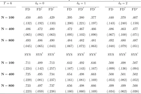
The results are provided in the table below. FD, FDy_{and FD denote the …rst-di¤erenced GMM}

estimators that utiliseZD,ZeD andZDe, respectively, as de…ned earlier in the paper, while SYS, SYSy

and SYS denote the system GMM estimators that utilise ZS,ZeS and ZSe, where ZeS is de…ned in

(58). Therefore, FD (SYS) makes use of the standard instruments that are available with respect to individual i, FDy _(SYSy_{) makes use of the spatials instruments with respect to the individuals}

which unit iis spatially correlated with, and FD (SYS ) combine the two sets of instruments.

Table 1. Performance in terms of mean point estimates and RMSE, = 0:5.

T = 6 0= 0 0= 1 0= 2

FD FDy FD FD FDy FD FD FDy FD

N=100 :450 :405 :429 :395 :380 :377 :440 :370 :407 (:132) (:192) (:133) (:200) (:221) (:197) (:143) (:240) (:159)

N=400 :486 :472 :480 :472 :467 :466 :486 :463 :477 (:065) (:092) (:063) (:095) (:102) (:090) (:067) (:100) (:071)

N=800 :493 :486 :490 :484 :482 :481 :492 :480 :487 (:045) (:065) (:043) (:067) (:072) (:063) (:048) (:079) (:051)

SYS SYSy SYS SYS SYSy SYS SYS SYSy SYS

N=100 :711 :489 :713 :642 :492 :646 :500 :498 :507 (:224) (:142) (:257) (:167) (:143) (:167) (:099) (:136) (:094)

N=400 :725 :495 :734 :654 :498 :663 :500 :501 :502 (:229) (:081) (:237) (:161) (:081) (:169) (:053) (:082) (:052)

N=800 :723 :497 :737 :656 :498 :666 :499 :499 :500 (:223) (:059) (:238) (:160) (:060) (:169) (:034) (:062) (:038)

As we can see, the performace of FD and FD is similar. In most cases FD has slightly less bias and slightly larger RMSE. This is not surprising; it is known that in …nite samples and with a …xed value of N, using a larger number of instruments results in a trade-o¤ between bias and e¢ciency. Of course, asymptotically the GMM estimator with the enlarged set of moment conditions is more e¢cient, providing that the additional moment conditions are not redundant. FDy _{is generally}

dominated by FD and FD both in terms of bias as well as RMSE. Its performance deteriorates with higher values of 0, which, however, is also the case for the remaining …rst-di¤erenced GMM

estimators. Intuitively, this is a weak instruments problem; as 0 increases the proportion of the

variance of the total disturbance that is due to the variance of the individual-speci…c e¤ects gets larger. Essentially, abusing the notation, for 0 ! 1 we have 2= 2" ! 1 and the instruments

become weak (see Blundell and Bond, 1998). The same intuition holds for the spatial instruments. Similarly to FD and FD , the performance of SYS and SYS is similar under all circumstances. However, both estimators are consistent only under mean-stationarity and they appear to exhibit a large upwards bias otherwise. SYSy_{, on the other hand, performs well under all situations and largely}

dominates SYS and SYS , unless the process is mean-stationarity. Importantly, SYSy _{appears to}

case SYSy_{uniformly dominates FD and FD under all circumstances. To save space we do not report}

these results. In the section below it will be demonstrated that the spatial moment conditions can be used to construct consistent GMM estimators in situations were the standard GMM estimators are not consistent.

4

Spatial and Factor Structure Dependence

In this section we will consider a panel autoregressive model in which the disturbance contains a common factor structure, such that

e

yit = yeit 1+ueit, j j<1,i= 1; :::; N,t= 1; :::; T,

e

uit = i+ 0i t+"it,"it= N

X

j=1

wij;N jt+ it,

where _t= ( _1t; _2t; :::; _nt)0 is a n 1vector of factors and i = ( 1i; 2i; :::; ni)0 is a n 1vector

of factor loadings. A similar structure is also studied by Pesaran and Tosetti (2011) and Chudik, Pesaran and Tosetti (2011). We make the following assumption regarding the factors and their loadings:

Assumption 4 (common factor component): (i) The random variables_f ri: 1 i N,1 r ng

are independently distributed with zero mean and …nite variance 2

r. Furthermore,sup1 i N;0 r n

E_j rij4+ <1for some >0. (ii) t is non-stochastic and has uniformly bounded elements,

such that _{k tk} c <_{1 8}t. (iii) The processes _f rig,f itgandf igare totally independent.

Assumption 4 is standard in factor analysis; see for example, Sara…dis, Yamagata and Robertson (2009) and Sara…dis and Wansbeek (2012). The zero mean assumption on the vector i is not

restrictive because the model can be expressed in terms of deviations from time-speci…c averages, which will eliminate the non-zero mean of i (e.g. Sara…dis and Robertson, 2009). The vector of

factors is treated as …xed and the factor loadings as random variables because the asymptotics apply for largeN,T…xed. Observe that iis correlated with the lagged dependent variable by construction

and cannot be eliminated using the …rst-di¤erence transformation because i is multiplicative with t, which is time-varying. One may think of the loadings in this context as re‡ecting di¤erent

sources of unobserved heterogeneity, the impact of which is not constant through time. Rewriting the model in vector form yields

e

yt= eyt 1+uet,uet= + t+PN t, (47)

where = ( 1; :::; N)0 is a N n matrix. Observe that eytcan be written as

e

yt= tey0+

1 t

1 +

t 1

X

=0

t +PN t 1

X

=0

t , (48)

and the initial observation is now given by y_e0 = 0 + 1PN 0+ 2 0. Therefore, eyt and eut can

be expressed as linear forms of the innovations , and :

e

yt= 0;t + IN 1;t + ( t PN) , (49)

and

e

ut= + IN 0t + e0t+1 PN , (50)

where _1;t = 2 t; t 1; :::; 0 is a 1 (T+ 1) row vector, = ( 0; :::; T)0 is a (T+ 1) n

matrix, =vec( 0_{)is anN 1row vector, while the remaining terms have been de…ned in Section}

2. Stacking (47)overt= 2; :::; T yields e

where _ey= (y_e0

2; :::;ye0T)

0

,_ey 1 = ey01; :::;ye0T 1

0

,_eu= (u_e0

2; :::;ueT0)0.

Similarly, taking …rst-di¤erences in(47) yields e

yt= eyt 1+ t+PN t. (52)

e

yt and uetcan be expressed as linear forms of the innovations as follows:

e

yt= 0;t + IN 2;t + ( t PN) , (53)

and

e

ut= IN 0t + (dt PN) , (54)

where _2;t = 2( 1) t 1;( 1) t 2; :::;( 1) 0;1 is a1 (t+ 1)row vector. Stacking the

column vectors in (52) overt= 2; :::; T yields e

y= ey 1+ u.e (55)

As shown by Sara…dis and Robertson (2009) for the case where = 0, the standard moment conditions that utilise instruments with respect to lagged values of yit 1 in the …rst-di¤erenced

equations and yit 1in the levels equations are invalidated under a factor structure in the residuals.

A similar result applies for ₆= 0 of course.5 Therefore both bD and bS as de…ned in(16) and (17)

respectively, are not consistent. However, as the following proposition demonstrates, the moment conditions that utilise instruments with respect to the individuals which unitiis spatially correlated with, remain valid. These moment conditions will be used to obtain consistent estimates of the structural parameter .

Proposition 6 Under Assumptions 1-4, the followingT(T 1)=2 moment conditions are valid in the …rst-di¤erenced model (55):

e

m_N;De( ) =N 1Ze_D0 ue_!p 0. (56) Furthermore, the following T 1 moment conditions are valid in the levels model (51):

e

m_N;Le( ) =N 1Ze_L0ue_!p 0. (57)

Proof. See Appendix A.

Observe that we have made no assumptions about mean-stationarity of the process. Indeed this assumption is always violated when there exists a common factor component because the mean of the process shifts every time period according to the value of _t. Therefore, one requires an estimator that does not rely on this assumption. De…ne

e

ZS

" e

ZD 0

0 ZeL

#

, (58)

and letA3;D;N and A3;S;N be sequences of possibly random, non-negative de…nite matrices of order

1;D 1;D, and 1;S 1;S, respectively. The following assumption is employed for the identi…cation

of :

Assumption 3(iii) (identi…cation of ): N 1Ze0

DZeD p

!Q_Ze

D,N

1_Ze0

D ye 1

p

!q_Ze

D ey 1,N

1_Ze0

SZeS p

! Q_Ze

S, , N

1_Ze0

Sey 1;S p

! q_Ze

Sey 1;S, all …nite matrices (vectors) with full column rank

(non-zero entries). A3;D;N and A3;S;N have full rank, such thatA3;D;N !p A3;D,A3;S;N !p A3;S.

5_{For the case of a degenerate factor structure, which takes the form of a singe individual-invariant time e¤ect, a}

Consider the following GMM estimators:

bDe(A3;D;N) =

h e

y0 ₁ZeDA3;D;NZeD0 ey 1

i 1h

e

y0 ₁ZeDA3;D;NZeD0 ey

i

, (59)

and

bSe(A3;S;N) =

h e

y0 _1;SZeSA3;S;NZeL0ye 1;S

i 1h

e

y0 _1;SZeSA3;S;NZeS0eyS

i

. (60)

The following theorem establishes the consistency and asymptotic normality of the above estimators under a factor structure and spatially correlated idiosyncratic components.

Theorem 7 Suppose Assumptions 1-4, and (56) hold true. Let 3;D;N =var

h_p

Nme_N;De( )i be a sequence of symmetric non-negative de…nite matrices with rank greater than or equal to _1;D, such that min( 3;D;N) c >0, and 3;D;N

p

! 3;D =asy:var

h_p

Nme_N;De( )i. The GMM estimator in

(59) is consistent and

p

N _{bDe !}d N 0;Ve_De , (61)

where

e

V_De =hq_Ze

D ye 1A3;Dq

0 e

ZD ey 1

i 1

q_Ze

D ye 1A3;D 3;DA3;Dq

0 e

ZD ey 1

h q_Ze

D ye 1A3;Dq

0 e

ZD ye 1

i 1

. (62)

In addition, suppose that (57)holds true and let 3;S;N =var

h_p

Nme_N;Le( )ibe a sequence of sym-metric non-negative de…nite matrices with rank greater than or equal to _1;S, such that min( 3;S;N)

c >0, and 3;S;N !p 3;S =asy:var

h_p

Nme_N;Le( )i. The GMM estimator in (60) is consistent and

p

N _{bSe !}d N 0;Ve_Se , (63)

where

e

V_Se=hq_Ze

Sey 1A3;Sq

0 e

ZSye 1

i 1

q_Ze

Sye 1A3;S 3;SA3;Sq

0 e

ZSye 1

h q_Ze

Sye 1A3;Sq

0 e

ZSey 1

i 1

.

Proof. See Appendix A.

The optimal GMM estimators are obtained by replacingA3;D;N,A3;S;N by consistent estimates

of _3;D;N1 and _3;S;N1 , respectively. As in Section (2), 3;D;N can be partitioned as

3;D;N =

2 6 4

3;22;D;N 3;2T;D;N

. ..

3;T2;D;N 3;T T;D;N

3 7 5,

where 3;ts;D;N = N 1EYt 20WfN uet ue0sYs 2. The pqth element of 3;ts;D;N is !3;pq;ts;D;N =

N 1Eye0

pWfN uet ues0WfNeyq. Therefore, from the proof of Proposition 6, equation (81), it is clear

that to obtain a consistent estimate of 3;D;N, one requires estimating the number of unobserved

factors and the factors themselves. For inference purposes, a consistent estimate of 3;D is required

even for a sub-optimal GMM estimator, as it is clear from(62). The same issue applies for 3;S;N. To

avoid this complication, the standard errors for the sub-optimal GMM estimators can be computed using spatial block bootstrapping (e.g. Hall, 1985 and Anselin, 1990). We investigate this approach in simulations.

5

A Simulation Study

5.1 Design

The underlying generating process is given by

yit= yit 1+uit, ,uit= i t+ N

X

j=1

wij;N jt+ it,i= 1; :::; N,t= 1; :::; T, (64)

wherewij;N is formed as in(41), i i:i:d:U[ 0:25;0:25], t i:i:d:N(0;1)and it i:i:d:N(0;1).

The performance of the estimators will depend on the proportion of 2

uattributed to the variance

of the common factor component hereafter this proportion is denoted by . Therefore, noticing that

2

u = 2 2 + 2 2 + 2 1 + 2 , (65)

and normalising 2 = 1, we have

2 ₌ (1 ) 2

1 + 2 (66)

We set = 0:5, which implies that 2 will change only according to since the value of 2 is …xed in the design. As the value of approaches unity, the impact of the factor component in the total error process increases. We choose the following values for :

8 > > < > > :

Low impact of factor structure onuit: = 1=3

Medium impact of factor structure onuit: = 1=2

Medium-to-high impact of factor structure onuit: = 2=3

High impact of factor structure on uit: = 3=4

We setT = 10, and we experiment between _{2 f}:2; :5; :8_gand N _{2 f}100;400;800_g. Notice that under a factor structure, mean-stationarity is always violated by construction because the mean shifts every time period according to the value of _t. To enhance transparency and save space, we simply set the initial value of the process as yi0 = i 0 +"i0. All experiments are based on 2,000

replications.

To compute empirical standard errors for the estimators, we use block bootstrapping. The algorithm can be outlined as follows: each individual i is assigned an equal probability of being selected with replacement. If unit i is selected, the complete time series of unit i is sampled to preserve the serial correlation structure of the data. The complete time series of uniti’s neighbours, as re‡ected on WN, are sampled as well. This process is repeated until the data set equals the

original size ofN. Once the sampling process is complete, estimates of the autoregressive parameter are obtained using the various methods employed in this simulation experiment. For the estimators that rely on spatial instruments, we make use of the spatial neighbours information, i.e. instruments are utilised with respect to the individuals, unit i is spatially correlated. The same procedure is followed over 200 bootstrapped samples, and the empirical standard errors of the estimators are computed in each replication.

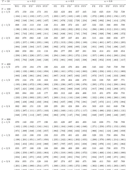
5.1.1 Results

Table A1 in the appendix reports mean bias, root mean square error and empirical size (nominal size is 5%) for the estimators employed in this study. W Gis the within-group estimator, FD (SYS) and FDy_(SYSy_{) denote the …rst-di¤erenced (system) GMM estimators that utiliseZ}

D (ZS) andZeD

(ZeS), respectively, as de…ned earlier in the paper.6

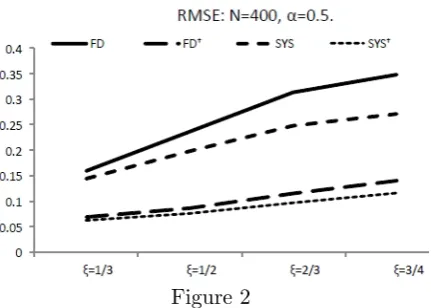
The performance of all estimators depends on the value of , and the size ofN. Speci…cally, as the value of increases for a given value of andN, the performance of the estimators deteriorates in terms of bias and RMSE. This is illustrated in Figure 2 for = 0:5,N = 400.

6_{For FD}y _{we setA3}

;D;N =N

1_e Z0

D(DD0 IN)ZeD, and similarly for FD, expect thatZeD is replaced byZD. For SYSy_{we setA3}

;S;N =N

1_e Z0

Figure 2

This is expected because higher values of imply that the invalidity of the instruments used with respect to unit i itself (utilised by FD and SYS) is magni…ed; for the estimators that make use of the spatial instruments, the increase in bias and RMSE is also intuitive because as the value of increases the contribution of the spatial component in the total error process, and thereby the correlation between the endogenous variable and the spatial instruments, decreases.

However, it is important to emphasise two points; …rstly, both FDy _{and SYS}y _uniformly

out-perform FD and SYS, respectively, in terms of RMSE. The same holds for bias, unless N is small. Secondly, as the value ofN increases, the bias and RMSE of FDy _{and SYS}y _{decreases considerably,}

which is natural as these estimators are consistent. This is not the case for the conventional estim-ators, FD and SYS, the performance of which does not improve with larger values of N. This is illustrated in Figure 3 below for = 1=3and = 3=4. Similar graphs apply for the remaining values of , not illustrated here.

Figure 3a Figure 3b

It is also worth mentioning that SYSy _{appears to outperform FD}y _{in terms of both bias and}

RMSE in all circumstances, with the relative di¤erence in performance increasing according to the value of .

In terms of empirical size, the results indicate that this is largely distorted for the conventional estimators, WG, FD and SYS, which is natural since these estimators exhibit large bias. The same applies to FDyand SYSywhenN is small. However, asN increases, size improves considerably and appears to converge to the nominal level, especially for SYSy_{, which contrary to the conventional}

6

Concluding Remarks

Error cross-sectional dependence is an increasingly popular research area in the analysis of panel data. This papers considers spatial dependence and factor structure dependence in dynamic panel data models. It is shown that under spatially correlated errors, an additional set of moment condi-tions arises in particular, instruments with respect to the individual(s) which unitiis correlated with. We demonstrate that these moment conditions remain valid when the errors contains a common factor component, in which case the standard instruments are invalidated. The resulting estimators are attractive because, aside from specifying a weighting matrix W, they are compu-tationally simple and provide consistent estimates of the structural parameters without requiring estimation of the number of unobserved factors, or the factors themselves. Simulation experiments show that the proposed estimators largely outperform the conventional ones, in terms of both bias and root mean square error. This result is even more pronounced as N becomes larger.

References

[1] Ahn, S. C., Lee, Y.H., Schmidt, P., 2001. Panel data models with multiple time-varying indi-vidual e¤ects, Mimeo.

[2] Ahn, S.C., Schmidt, P., 1995. E¢cient estimation of models for dynamic panel data. Journal of Econometrics 68, 5-28.

[3] Anderson, T.W., Hsiao, C., 1981. Estimation of dynamic models with error components. Journal of the American Statistical Association 76, 598-606.

[4] Anselin, L., 1990. Some Robust Approaches to Testing and Estimation in Spatial Econometrics. Regional Science and Urban Economics 20, 141-163.

[5] Anselin, L., 2001. Spatial Econometrics. In: Baltagi, B.H. (Eds.), A Companion to Theoretical Econometrics. Blackwell Publishing, pp. 310-330.

[6] Arellano, M., 2003. Panel Data Econometrics. Oxford University Press, Oxford.

[7] Arellano, M., Bond, S., 1991. Some tests of speci…cation for panel data: Monte carlo evidence and an application to employment equations. Review of Economic Studies 58, 277-297.

[8] Arellano, M., Bover, O., 1995. Another look at the instrumental variable estimation of error-Component models. Journal of Econometrics 68, 29-51.

[9] Bai, J., 2009. Panel data models with interactive …xed e¤ects. Econometrica 77, 1229-1279.

[10] Baltagi, B., Bresson, G., Pirotte, A., 2007. Panel unit root tests and spatial dependence. Journal of Applied Econometrics 22, 339-360.

[11] Blundell, R., Bond, S., 1998. Initial conditions and moment restrictions in dynamic panel data models. Journal of Econometrics 87, 115-143.

[12] Bover, O., Watson, N., 2005. Are there economies of scale in the demand for money by …rms? Some panel data estimates. Journal of Monetary Economics 52, 1569-1589.

[13] Breusch, T., Qian, H., Schmidt, P., Wyhowski, D., 1999. Redundancy of moment conditions. Journal of Econometrics 91, 89-111.

[15] Conley, T.G., 1999. GMM estimation with cross-sectional dependence. Journal of Econometrics 92, 1-45.

[16] Fingleton, B., 2008. A generalized method of moments estimator for a spatial model with moving average errors, with application to real estate prices. Empirical Economics 34, 35-57.

[17] Goldberger, A.S., 1972. Structural equation methods in the social sciences. Econometrica 40, 979-1001.

[18] Hall, P., 1985. Resampling a coverage pattern. Stochastic Processes and their Applications 20, 231-246.

[19] Hsiao, C., Tahmiscioglu, A.K., 2008. Estimation of dynamic panel data models with both individual and time speci…c e¤ects. Journal of Statistical Planning and Inference 138, 2698-2721.

[20] Jöreskog, K.G., Goldberger, A.S., 1975. Estimation of a model with multiple indicators and multiple causes of a single latent variable. Journal of the American Statistical Association 70, 631-639.

[21] Kapoor, M., Kelejian, H.H., Prucha I.R., 2007. Panel data models with spatially correlated error components. Journal of Econometrics 140, 97-130.

[22] Kelejian, H., Prucha I.R., 2010. Speci…cation and estimation of spatial autoregressive models with autoregressive and heteroskedastic disturbances. Journal of Econometrics 157, 53-67.

[23] Lee, L., 2007. GMM and 2SLS estimation of mixed regressive, spatial autoregressive models. Journal of Econometrics 137, 489-514.

[24] Lee, L. Yu, J., 2010. E¢cient GMM estimation of spatial dynamic panel data models with …xed e¤ects, Mimeo.

[25] Moon, H.R., Perron, B., 2004. E¢cient estimation of the SUR cointegrating regression model and testing for purchasing power parity. Econometric Reviews 23, 293-323.

[26] Mutl, J., 2006. Dynamic panel data models with spatially correlated disturbances. PhD Thesis, University of Maryland, College Park.

[27] Pesaran, H., 2006. Estimation and inference in large heterogeneous panels with a multifactor error structure. Econometrica 74, 967-1012.

[28] Pesaran, H., Tosetti, E., 2011. Large panels with common factors and spatial correlations. Journal of Econometrics 161, 182-202.

[29] Phillips, P., Sul, S., 2003. Dynamic panel estimation and homogeneity testing under cross-sectional dependence. The Econometrics Journal 6, 217-259.

[30] Robertson, D., Symons, J., 2007. Maximum likelihood factor analysis with rank de…cient sample covariance matrices. Journal of Multivariate Analysis 98, 813-828.

[31] Sara…dis, V., Yamagata, T., 2010. Instrumental variable estimation of dynamic linear panel data models with defactored regressors under cross-sectional dependence. Mimeo.

[32] Sara…dis, V., Yamagata, T., Robertson, D., 2009. A test of error cross-sectional dependence for a linear dynamic panel model with regressors. Journal of Econometrics 148, 149-161.

Appendix A

The(t 1)thblock ofN 1Ze0

D ", fort= 2; :::; T, whereZeD =diag fWNY0;fWNY1; :::;fWNYT 2

and WfN =WN +WN0 , withWfN0 = (WN +WN0 )

0

=W0

N+WN =WfN, is given by

N 1 WfNYt 2

0

"t = N 1

2 6 6 6 6 4

y0

0WfN "t

y0

1WfN "t

.. . y0

t 2fWN "t

3 7 7 7 7 5

= N 1

2 6 6 6 6 6 6 4

0 0

0dt PN0 WfNPN + 0;s 0 dt WfNPN

0 0

1dt P_N0 WfNPN + 0;s 0 dt WfNPN

.. .

0 0

t 2dt P_N0 fWNPN + 0;s 0 dt WfNPN

3 7 7 7 7 7 7 5 ,

since, using (4)and (5), we have y0

sWfN "t = 0 0s PN0 + 0;s 0 fWN[(dt PN) ]

= 0 0_s P_N0 WfN(dt PN) + 0;s + 0;s 0WfN(dt PN)

= 0 0_s P_N0 1 WfN (dt PN) + 0;s 0 1 WfN (dt PN)

= 0 0_sdt PN0 WfNPN + 0;s 0 dt WfNPN . (67)

The(t 1)th block ofN 1_Z0

D "is identical except thatWfN is replaced by IN, theN N identity

matrix.

Similarly, using(6) and(8), the(t 1)th block of Ze0

lucan be written as

y0_{t 1}fWNut = 0 0t 1 PN0 + 0;t 1 0 fWN e0t+1 PN +

= 0 0_{t 1} P_N0 WfN e0t+1 PN + 0 0t 1 PN0 fWN

+ _{0;t 1} 0WfN e0t+1 PN + 0;t 1 0WfN

= 0 0_{t 1}e0_t+1 P_N0 fWNPN + 0 0t 1 PN0 fWN

+ _{0;t 1} 0 _e0

t+1 WfNPN + 0;t 1 0WfN . (68)

The (t 1)th block of Z0

Lu is identical except thatWfN is replaced by IN.

Furthermore, the(t 1)th block of N 1_Ze0

D y 1, for t= 2; :::; T, is

N 1 WfNYt 2

0

y ₁ =N 1

2 6 6 6 6 4

y0

0WfN yt 1

y0

1WfN yt 1

.. . y0

t 2WfN yt 1

3 7 7 7 7 5,

where

y0_sfWN yt 1 = 0 0s PN0 + 0;s 0 fWN t 1 PN + 0;t 1

= 0 0_{s t 1} P_n0WfNPN + 0;t 1 0 0s PN0 WfN

while using (4)and (8), the(t 1)th block of N 1_Ze0

Ly 1 can be written as

N 1 y0_{t 1}WfNyt 1 = 0 0t 1 PN0 + 0;t 1 0 WfN t 1 PN + 0;t 1

= 0 0_{t 1 t 1} P_N0 WfNPN + 0;t 1 0 t 1 WfNPN

+ _{0;t 1} 0 0_{t 1} P_N0 WfN + 0;t 1 0;t 1 0WfN . (70)

We de…ne the following terms:

1;st;N N 1y0s "t;

2;t;N N 1 y0t 1ut;

3;st;N N 1y0sfWN "t;

4;t;N N 1 y0t 1WfNut;

5;st;N N 1y0sfWN yt 1;

6;t;N N 1 y0t 1WfNyt 1.

PROOF OF PROPOSITION 1

We need to show that (i) E _1;st;N = 0, E 2_{1;st;N !} 0 as N _{! 1} for t = 2; :::; T, s t 2, and (ii) E _2;t;N = 0,E 2_{2;t;N !}0 asN _{! 1}for t= 2; :::; T. This is entirely straightforward from the proof in Proposition 3 by replacing WfN by IN and using the mean-stationarity assumption for

2;t;N, which implies that 0;t 1 = 08t. The claims in Proposition 1 then follow from Chebychev’s

inequality. QED

PROOF OF PROPOSITION 3

Firstly, we will show that (i)E _3;st;N = 0,E 2_{3;st;N !}0 as N _{! 1} fort= 2; :::; T, s t 2, and (ii)E _4;t;N = 0,E 2_{4;t;N !}0asN _{! 1}fort= 2; :::; T.

We have

E _3;st;N = N 1Eh 0 0_sdt PN0 fWNPN + 0;s 0 dt WfNPN

i

= N 1trh 0_sdt PN0 WfNPN E 0

i

+ _0;strh dt WfNPN E 0

i

= N 1trh 0

sdt PN0 WfNPN

i

, (71)

since E 0 _{= 0 under the maintained assumptions. Observe that} 0

sdt is a (T + 1) (T + 1)

matrix that contains zeros on the main diagonal s t 2. Therefore, 0_sdt Pn0fWNPn is a

N(T + 1) N(T+ 1) matrix with zeros on the main diagonal and by Lemma 9 it has uniformly bounded row and column sums, setting _s0dt = H and PN0 WfNPN = C1;N. In addition, is a

N(T + 1) N(T+ 1) diagonal matrix under the maintained assumptions with uniformly bounded elements. Hence, tr 0_sdt P_N0 PN = 0 by Lemma 10(i), setting 0sdt P_N0 WfNPN = C₁0_;`N

and =D1;`N, with`=T + 1. Therefore, E 3;st;N = 0.

The variance of _3;st;N equals

E 2_3;st;N = N 2E_fh 0 0

sdt PN0 WfNPN + 0;s 0 dt WfNPN

i

h

0 _d0

t s PN0 WfNPN + 0;s 0 dt WfNPN

i

g

= N 2Eh 0 0_sdt PN0 WfNPN 0 d0t s PN0 WfNPN

i

+N 2 ₀2_;sEh 0 dt WfNPN 0 d0t PN0 fWN

i

+N 22 _0;sEh 0 0_sdt PN0 fWNPN 0 d0t PN0 fWN

i

The …rst term on the right-hand side of the last equality above equals

N 2Eh 0 0_sdt PN0 WfNPN 0 d0s t PN0 WfNPN

i

=N 22tr C₁0_{;`N</sub> C<sub>1</sub>0<sub>;`N}0 ,

with`=T+ 1. This follows from Lemma 11(i) and the fact thatc0

ii;1;`N = 0fors t 2. Given this

property and since is diagonal, it follows from Lemma 10(iii) thatN 22tr C₁0_;`N C00

1;`N =

o(1). The second term is

N 2Eh 0 dt WfNPN 0 d0t fWNPN0

i

= N 2trEh dt fWNPN 0 d0t PN0 fWN 0

i

= N 2trh dt WfNPN d0t PN0 WfN

i

= N 2trh dt WfNPN d0t PN0 WfN (1 )

i

= N 2trh dt PNWfN d0t PN0 WfN

i

. (73)

By Lemma 9 the row and column sums of dt fWNPN and d0t PN0 WfN are uniformly

bounded. Furthermore, is a diagonal matrix with uniformly bounded diagonal entries. As a res-ult,N 2_trh _d

t WfNPN d0t PN0 fWN

i

=o(1)by Lemma 10(ii), setting dt WfNPN =

C0

2`N, =D1;`N and d

0

t PN0 fWN =C₃0_`N The third term equals zero by Lemma 11(iv). It

follows from Chebychev’s inequality that N 1_y0

sWfN "t p

!0. For _4;st;N we have, using(6)and (8),

E _4;t;N = N 1Eh 0 0_{t 1}e0_t+1 P_N0 WfNPN

i

+N 1Eh 0 0_{t 1} P_N0 WfN

i

+ _{0;t 1}N 1Eh 0 e0_t+1 fWNPN

i

+ _{0;t 1}N 1Eh 0WfN

i

= N 1trh 0

t 1e0t+1 PN0 WfNPN E 0

i

+N 1trh 0

t 1 PN0 WfN E 0

i

+ _{0;t 1}N 1trh e0_t+1 WfNPN E 0

i

+ _{0;t 1}N 1trhfWNE 0

i

. (74)

Under the maintained assumptions E 0 _{= 0. In addition, both} 0

t 1e0t+1 PN0 WfNPN and WfN

have uniformly bounded row and column sums and contain zeros on the main diagonal. Therefore, by Lemma 10(i) E _4;t;N = 0. Notice that the expression for N 1 y0

t 1ut is obtained by replacing

f

WN by the identity matrix. In this case the last term is zero only if 0;t 1 = 0, which is satis…ed

under mean-stationarity of the process. The variance of _4;st;N equals

E 2_4;t;N = N 2E_f[ 0 0_{t 1}e0_t+1 P_N0 WfNPN + 0 0t 1 PN0 WfN

+ _{0;t 1} 0 e0_t+1 WfNPN + 0;t 1 0fWN ]

[ 0 et+1 t 1 PN0 fWNPN + 0 t 1 fWNPN

= N 2Eh 0 0_{t 1}e0_t+1 P_N0 WfNPN 0 t 1et+1 PN0 WfNPN

i

+N 22Eh 0 0_{t 1}e0_t+1 P_N0 WfNPN 0 t 1 WfNPN

i

+N 22 _{0;t 1}Eh 0 0_{t 1}e0_t+1 P_N0 WfNPN 0 et+1 PN0 WfN

i

+N 22 _{0;t 1}Eh 0 0_{t 1}e0_t+1 P_N0 WfNPN 0fWN

i

+N 2Eh 0 0_{t 1} P_N0 WfN 0 t 1 WfNPN

i

+N 22 _{0;t 1}Eh 0 0_{t 1} P_N0 WfN 0 et+1 PN0 WfN

i

+N 22 _{0;t 1}Eh 0 _t0 ₁ P_N0 WfN 0WfN

i

+N 2 _0;t2 ₁Eh 0 e0_t+1 WfNPN 0 et+1 PN0 WfN

i

+N 22 _0;t2 ₁Eh 0 e0_t+1 WfNPN 0WfN

i

+N 2 _0;t2 ₁Eh 0fWN 0WfN

i

= N 22tr C₄0_{;`N</sub> C<sub>4</sub>0<sub>;`N}0 +N 22 _{0;t 1}trhC₄0_;`N WfN

i

+N 2tr G1;`N G01;`N +N 22 0;t 1tr G1;n C50;`N

+N 22 _0;t2 ₁tr C₅0_{;`N</sub>0 C<sub>5</sub>0<sub>;`N} +N 22 _0;t2₁trhfWN fWN

i ,

where C₄0_;`N = 0

t 1e0t+1 PN0 WfNPN ,G1;n = 0t 1 PN0 WfN ,C50;`N = et+1 PN0 fWN , using

Lemma 11 repeatedly. Finally, by Lemma 10(iii)-(iv) it follows immediately that E 2_4;t;N = o(1)

and so N 1 _y0

t 1WfNut!p 0 by Chebychev’s inequality.

Next, we will show that (i) E _5;st;N = qst;d 6= 0, in general, E 25;st;N ! 0 as N ! 1 for

t= 2; :::; T,s t 2, and (ii) E _6;t;N =qt;s= 06 , in general,E 26;t;N !0asN ! 1fort= 2; :::; T.

The expected value ofE _5;st;N, using(4) and (8), is given by

E _5;st;N = N 1E 0 0_s P_N0 + _0;t 0 fWN t 1 PN + 0;t 1

= N 1Eh 0 0_{s t 1} P_N0 WfNPN

i

+ _{0;s 0;t 1}N 1Eh 0WfN

i

+ _{0;t 1}N 1Eh 0 0_s P_N0 WfN

i

+ _0;sN 1Eh 0 _{t 1} WfNPN

i

= N 1trh 0_{s t 1} P_N0 WfNPN E 0

i

+ _{0;s 0;t 1}N 1trhWfNE 0

i

+N 1 _{0;t 1}trh _s0 P_N0 WfN E 0

i

+N 1 _0;strh _{t 1} fWNPN E 0

i

= N 1trh 0_{s t 1} P_N0 WfNPN

i

=qst;D, (75)

since E 0 _{= E} 0 _{= 0 under the maintained assumptions. We have also used the fact that}

trhWfNE 0

i

= trhfWN

i

= 0 from Lemma 10(i), given that WfN contains zeros on the main

diagonal and is diagonal. Observe that qst;D 6= 0 in general, unless = 0, in which case

PN = IN ) PN0 fWNPN = WfN. As a result, the kronecker product matrix contains zeros on the

main diagonal and so qst;D = 0. Therefore, the spatial instruments are not correlated with the