Aggregating Density Estimators: An Empirical Study
Mathias Bourel1,2, Badih Ghattas2 1
Instituto de Matemática y Estadística, Facultad de Ingeniería, Universidad de la República, Montevideo, Uruguay 2
Institut de Mathématiques de Luminy, Université d’Aix-Marseille, Marseille, France Email: [email protected],[email protected]
Received June 20, 2013; revised July 20, 2013; accepted July 27,2013
Copyright © 2013 Mathias Bourel, Badih Ghattas. This is an open access article distributed under the Creative Commons Attribution License, which permits unrestricted use, distribution, and reproduction in any medium, provided the original work is properly cited.
ABSTRACT
Density estimation methods based on aggregating several estimators are described and compared over several simula- tion models. We show that aggregation gives rise in general to better estimators than simple methods like histograms or kernel density estimators. We suggest three new simple algorithms which aggregate histograms and compare very well to all the existing methods.
Keywords: Machine Learning; Histogram; Kernel Density Estimator; Bagging; Boosting; Stacking
1. Introduction
Ensemble learning or aggregation methods are among the most challenging recent approaches in statistical learning. In a supervised framework, the main goal is to estimate a function using a data set of independent ob- servations of both variables x
:
f X Y
X and Ensemble learning constructs several such estimates 1
yY.
, , M
g g
1, , M, which are often called weak learners, and combines them to obtain the aggregated model f g g g
where g may be a simple or a weighted average whensuch as for regression, or a simple or a weighted majority voting rule when
Y
1, ,J
Y such as for classification. In this framework, Bagging ([1]), Boosting ([2]), Stacking ([3]), and Random Forests ([4]) have been declared to be the best of the shelf classifiers achieving very high performances when tested over tens of various datasets selected from the machine learning benchmark. All these algorithms had been designed for supervised learning, and sometimes initially restricted to regression or binary classification. Several extensions are still under study: multivariate regression, multiclass learning, and adaptation to functional data or time series.
Very few developments exist for ensemble learning in the unsupervised framework, clustering analysis and den- sity estimation. Our work concerns the latter case which may be seen as a fundamental problem in statistics. Among the latest developments, we found some exten- sions of Boosting ([2]) and Stacking ([5]) to density es- timation. The existing methods seem to be quite complex, often combining kernel density estimators and whose
parameters seem to be arbitrary. In particular, most of the methods combine a fixed number of weak learners.
In this paper we show extensive simulations that ag- gregation gives rise to effective better estimates than sim- ple classical density estimators. We suggest three simple algorithms for density estimation in the same spirit of bagging and stacking, where the weak learners are histo- grams. We compare our algorithms to several algorithms for density estimation, some of them are simple like His- togram and Kernel Density Estimators (Kde) and others rather complex like stacking and boosting, which will be described in details. As we will show in the experiments, although the accuracy of our algorithms is not system- atically higher than other ensemble methods, they are simpler, more intuitive and computationally less expen- sive. Up to our knowledge, the existing algorithms have never been compared over a common benchmark simula- tion data.
Aggregating methods for density estimation are de- scribed in Section 2. Section 3 describes our algorithms. Simulations and results are given in Section 4 and con- cluding remarks and future work are described in Section 5.
2. A Review of the Existing Algorithms
In this Section we review some density estimators ob- tained by aggregation. They may be classified in two ca- tegories depending on the aggregation form.
1 M
M m m
m
f x g
x (1)where m and gm is typically a parametric or non
parametric density model, and in general different values of m refer typically to different parameters values in the parametric case or different kernels or different band- widths for a chosen kernel for the kernel density estima- tors.
The second type of aggregation is multiplicative and is based on the ideas of high order bias reduction for kernel density estimation as in [6]. The aggregated density es- timator has the form:
1 M M m m mf x g
x (2)2.1. Linear or Convex Combination of Density Estimators
This kind of estimators (1) has been used in several works with different construction schemes.
In [7-9] the weak learners gm are introduced sequen-
tially in the combination. At step m, gm is a density
selected among a fixed class H and is chosen to ma- ximize the log likelihood of
1
1
,
m m m
f x f x g x 0,1 (3) In [8], gm is selected among a non parametric family
of estimators, and in [7,9], it is taken to be a Gaussian density or a mixture of Gaussian densities whose para- meters are estimated. Different methods are used to esti- mate both density gm and the mixture coefficient .
In [7], gm is a Gaussian density and the log likelihood
of (3) is maximized using a special version of Expecta- tion Maximization (EM) taking into account that a part of the mixture is known.
The main idea underlying the algorithms given by [8,9] is to use Taylor expansion around the negative log like- lihood that we wish to minimize:
1
1
log m i log m i m i
i i i m i
g x
f x f x
f x
where T
x1,,xn
is the data set. Thus, minimizing theleft side term is equivalent to maximizing
1
m i
i m i
g x
f x
,and the output of this method converges to a global minimum.
All the algorithms described above are sequential and the number of weak learners aggregated may be fixed by the user.
In [5], Smith and Wolpert used stacked density esti- mator applying the same aggregation scheme as in stacked regression and classification ([10]). The M
densities estimators g1,,gM are fixed in advance
(KDE with different bandwidths). The data set
x1, ,xn
T is divided into V cross validation sub- sets L1,,LV. For v1,,V, denote L v L\Lv. The M models g1,,gM are fitted using the training
samples and the obtained estimates are denoted by for all
1
, ,
L L V 1, , m M.
v
These models are then evaluated over the test samples getting the vectors
1, , V
L L
v
mg L
n M
for put
within a
1, , , 1, m M v ,V
block matrix:
1 1 1
1 1 2 1 1
2 2 2
1 2 2 2 2
1 2
M
M
v v v
v v M v
g L g L g L
g L g L g L
A
g L g L g L
This matrix is used to compute the coefficients
1, , M
of the aggregated model (1) using the EM al- gorithm. Finally, for the output model, we re-estimate the individual densities g1,,gM from the whole data.
This method has been compared with other algorithms including the best single model obtained by cross-vali- dation, the best single model obtained over a test sample and a uniform average of the different Kde models. It is shown that stacking outperforms these methods for dif- ferent criteria: log likelihood, L1 and L2 performance mea-
sures (for the two last criteria use the true density).
In [11], Rigollet and Tsybakov fixed the densities
1, , M
g g in advance like for stacking (Kde estima- tors with different bandwidths). The dataset is split in two parts. The first sample is used to estimate the den- sities gm, whereas the coefficients m are optimiz-
ed using the second sample. The splitting process is repeated and the aggregated estimators for each data split are averaged. The final model has the form
1 s
M
s S M
f x g
S
xs m
(4)
where S is the set of all the splits used and
1 ˆ M s M m mg x g
x (5)is the aggregated estimator obtained from one split s of the data, ˆs
m
g is the individual kernel density function es- timated over the learning sample obtained from the split s. This algorithm is called AggPure. The authors compared their algorithm using different choices for the Kde’s bandwidth that we describe in the simulations section. Oracle inequalities and risk bounds are given for this es- timator.
2.2. Multiplicative Aggregation
tion is the one described in [12] called BoostKde. It is a sequential algorithm where at each step m the weak lear- ner is computed as follows:
1 ˆ n m i m iw i x x
g x K
h h
(6)where K is a fixed kernel, h its bandwidth, and wm
i theweight of observation i at step m. Like for boosting, the weight of each observation is updated by
1 ˆ log ˆ m im m i
m i
g x
w i w i
g x
(7)
where ˆ i
m
i jm i
j i
x x
w i
g x K
h h
The output is given by
1 ˆ M M m mf x C g x
(8)where C is a normalization constant.
Using several simulation models the authors explore different values for the bandwidth h minimizing the Mean integrated Square Error (MISE) for few values of M. They show that a bias reduction is obtained for M = 2 but it is not clear how the algorithm behaves for more than two steps.
3. Aggregating Histograms
We suggest three new density estimators obtained by li- near combination like in (1), all of them use histograms as weak learners. The first two algorithms aggregate ran- domized histograms and may be parallelized. The third one is just an adaptation of Stacking using histograms in- stead of kernel density estimators.
The first algorithm is similar to Bagging ([1]). Given a data set T
x1,,xn
,M
and an integer L, at each step of the algorithm a bootstrap sample of T is generated and used to construct an histogram m
1,
m
g with L
equally spaced breakpoints. The output of this method is an average of the M histograms. We will refer to this algorithm as BagHist and it is detailed in Figure 1.
The second algorithm, AggregHist, works as follows. Consider the data set T
x1,,xn
and an integer L.1. Let T the original sample and L an integer. 2. For m1,,M:
a Let Tm be a booststrap sample of T.
b Set gmto be the histogram constructed over T
m
with L equispaced breakpoints.
3. Output:
1 M
M m m
m f x g x
0 g
ed
[image:3.595.55.289.203.329.2]be the histogram obtained over T using
Figure 1. Bagging histograms (BagHist).
Let equally
spac breakpoints denoted byB
b1,,bL
. We de- note by h bl bl1 for all l L andwidthof 0
2,, the b
g . At each step m1,,M add a random uni noise
we
form l m, U
ach breakpoint andconstruct an hist
0,
m
h to e ogram g
tp
using T and the new set of breakpoints. The final ou ut is an average of the histo- grams g1,,gM. The algorithm is detailed in Figure 2.
The value of the parameter L used for AggregHist and
Ba
alled StackHist
w
resent the simulations we have done
4.1. Models Used for the Simulations
ve referenced
gHist will be optimized and the procedure used for that will be described in the next Section.
Finally, we introduce a third algorithm c
here we replace in the stacking algorithm the six kernel density estimators by histograms with different number of breakpoints.
4. Experiments
In this Section we p
to compare all the methods described in Section 2 toge- ther with our three algorithms. We consider several data generating models we have found in the literature. We first show how our algorithms adjust quite well for the different models, and that the adjustment error decreases monotonically with the numbers of histograms used. Fi- nally we will compare our methods with ensemble me- thods for density estimation like Stacking, AggPure,
BoostKde which aggregated non parametric density es- timators. All these aggregating methods are compared to optimized Histogram (Hist) and Kde using different band- width optimization approaches.
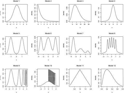
Twelve models found in the papers we ha
are used in our simulations. We denote them by M1,···,
M12 and we group them according to their difficulty level.
Some standard densities used in [11,12]: (M1)standard Gaussian density
N
(
0
,
1
)
, (M2)standard exponential density, (M3)a Chisquare density102 ,1. Let T the original sample, fix an integer L and construct the histogram g0 built over T, Bb1,,bL the equally
spaced breakpoints of g0 and h bl bl1. 2. For m1,,M:
a Consider * *
1, ,
m
L
B b b the randomly modified set of
breakpoints where *
, , ~, 0,
l l l m l m b b U h
b We compute ˆgmthe histogram over T using these new
breakpoints.
3. Output:
1
M
M m m
m f x g x
[image:3.595.63.279.627.720.2]
taken from [5,12]:
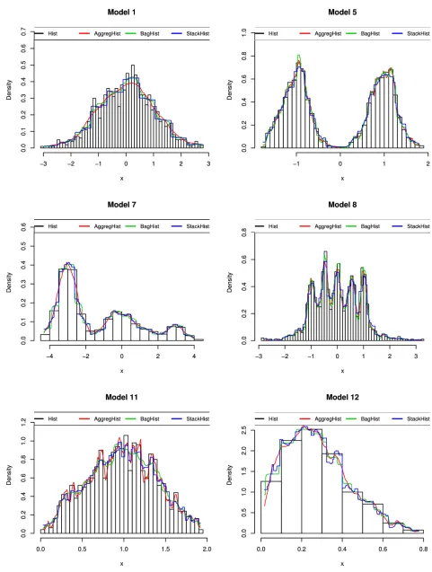
(M4)a student density t4, and StackHist (blue curve) for n = 1000 observations and M = 150 histograms for the two first algorithms. A simple histogram is shown together with the three estimates. For
StackHist we aggregate six histograms having 5, 10, 20, 30, 40 and 50 equally spaced breakpoints and a ten fold cross validation is used. Both AggregHist and BagHist
give more smooth estimators than StackHist. Some Gaussian mixtures
(M5) 0.5N
1, 0.3
0.5N
1, 0.3
,(M6)
.25N
3, 0.5
:
ensity,
ighly inhomogeneous
our study two simple models
ma- xi
eta density with parameters 2 and 5. e, and fo
some models, the estimator ob- ta
0.25N 3, 0.5 0.5N 0,1 0
(M7) 0.55N
3, 0.5
0.35N
0,1 0.1N
3, 0.5an mixtures used in [11] and taken from [13] Gaussi
(M8)the Claw density, (M9)the Smooth Comb d
(M10)is a mixture density with h
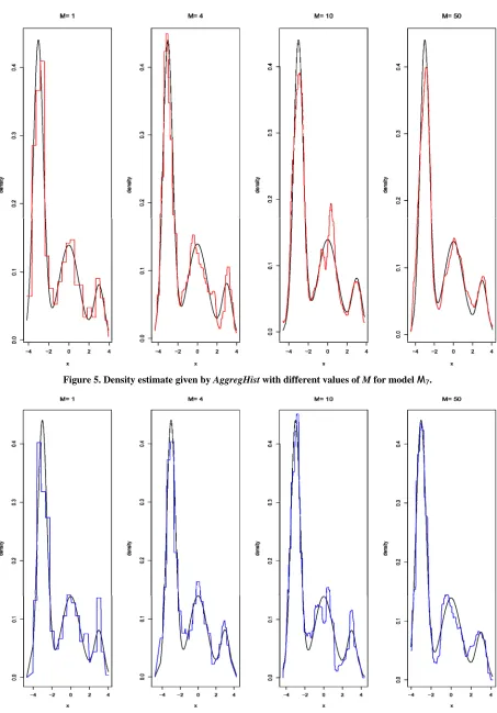
Figures 5 and 6 show the adjusted densities obtained from AggregHist and BagHist when increasing the num- ber M of histograms for model M7.
smoothness as in [12]
Finally we include in
4.2. Tuning the Algorithms
known to be challenging for density estimators: (M11) a triangular density with support [0,1] and mum at 1,
(M12)the b
All the simulations are done with the softwarR
[image:4.595.61.539.356.716.2]r models M8 and M9 we use the benchden package.
Figure 3 shows the shape of the densities we have used to generate the data sets.
Figure 4 shows, for
We compare the following algorithms AggregHist, Bag- Hist, StackHist, Stacking, AggPure and BoostKde with some classical methods like Hist and Kde.
For AggregHist and BagHist we fix the number of histograms to M = 200. The number of breakpoints is optimized testing different values over a fixed grid of 10, 20 and 50 equally spaced breakpoints. The optimal value retained for each model is the one which maximizes the log likelihood over 100 independent test samples drawn ined using AggregHist (red curve), BagHist (green curve)
Figure 5. Density estimate given by AggregHist with different values of M for model M7.
om the correspon
ha
mators are aggre-
aggre-
use 5 steps for the algorithm ag-
some co
ble 1. Optimal number of breakpoints used for Hist and
fr ding model. We optimize the number the Silverman’s rules of thumb ([14]) using factor 1.06
N an act 0. rd
.
The performance of each estimator is evaluated using the d Squared Error (MISE):
(Kde rd) d f or 9 (KdeN 0), of breakpoints of the histogram in the same way as for
our algorithms. These optimal values are given in Table 1 for differents values of n (100, 500 and 1000). We denote the optimal number of breakpoints LH, LBH and
LAH for Hist, BagHist and AggregHist respectively. To make the comparisons as faithful as possible
the unbiased cross-validation rule (KdeUCV, [15]),
the Sheater Johns plug-in method (KdeSJ, [16,17]). These choices are described in details in the appendix
4.3. Results
, we ve used for the other methods the same values sug- gested by their corresponding authors:
For Stacking, six kernel density esti Mean Integrate
2ˆ ˆ d
MISE f x E f x f x x
(9)gated, three of them use Gaussian kernels with fixed bandwidths h = 0.1, 0.2, 0.3 and the others use train- gular kernels with bandwidths h = 0.1, 0.2, 0.3. The number of cross validation samples is V = 10.
For AggPure six kernel density estimators are
ˆ
f f
where is the true density and its estimate. It is computed as the average of the integrated squared error
ˆ
ˆ
2dISE f x
f x f x x (10)over 100 Monte Carlo simulations. gated having bandwidths 0.001, 0.005, 0.01, 0.05, 0.1
and 0.5. Instead of the quadratic algorithm used by the authors in [11], we optimize the coefficients of the linear combination with the EM algorithm. The final estimator is a mean over |S| = 10 random splits of the original data set.
For BoostKde, we
For the same simulations, we have als
imization is equiva-
on
o computed the log likelihood criterion whose max
lent to reducing the Kullback-Leibler divergence between the true and the estimated densities (see P. Hall, “On Kull- back-Leibler loss and density estimation”, Ann. Stat., Vol. 15, 1987). The results obtained using this criterion are unstable due to numerical approximation of the log like- lihood for small values of the densities. In particular the histogram has very good performance with respect to the log likelihood when compared to all the other methods. This is due to the fact that when computing the log like- lihood we omit the points i for which f xˆ
i equals zero,and such points appear much more for the histogram than for the other methods. For all these reas s we do not report these results.
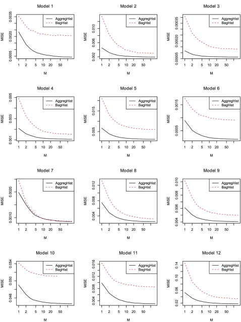
Figure 7 shows how the MISE varies when increasing the number of histograms in AggregHist and BagHist. For all
gregating kernel density estimators whose bandwidths are optimized using Silverman rule of thumbs (see
Appendix). Normalization of the output is done using numerical integration. Extensive simulations we have done using BoostKde showed that more steps give rise to less accurate estimators and unstable results. For Kde we use a standard gaussian kernel and mmon data driven bandwidth selectors:
Ta
our algorithms for each model and for each value of n.
n = 100 n = 500 n = 1000
the models, the adjustment error decreases significant- ly for the first 100 iterations. In most of the cases Ag- gregHist gives a better estimate than BagHist.
Table 2 shows the execution time for AggregHist,
BagHist, Stacking and AggPure for n = 2000. The other alg
Model
LH LBH LAH LH LBH LAH LH LBH LAH
M1 50 50 10 50 10 10 50 20 10
M2 50 50 50 50 50 50 50 50 50
M3 50 50 10 50 50 20 50 50 20
M4 50 50 20 50 50 50 50 50 50
M5 50 50 10 50 50 20 50 50 20
M6 50 10 10 20 20 20 20 20 20
M7 50 10 10 50 20 20 50 20 20
M8 50 50 50 50 50 50 50 50 50
M9 50 50 20 50 50 50 50 50 50
M10 50 50 50 50 50 50 50 50 50
M11 50 10 10 10 10 10 20 20 10
M12 50 10 10 20 20 10 20 20 20
orithms need much less time as they combine very few simple estimators and do not use any resampling. Computing time is significantly lower for our algorithms.
We compare now all the algorithms cited above over the twelve models using n = 100, n = 500 and n = 1000. For AggregHist and BagHist we use M = 200 histograms.
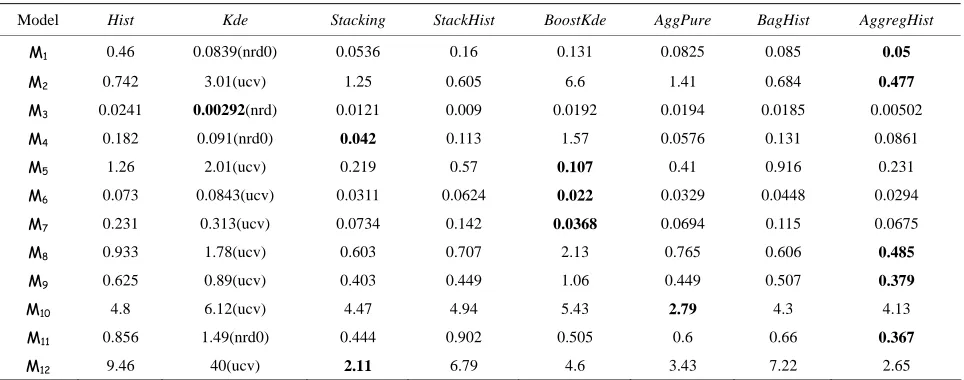
Tables 3 to 5 summarize the results for each value of n =
100, 500 and 1000. For each model and each method we give the average of 100 × MISE over 100 Monte Carlo simulations. For the Kde we kept the best result among the four choices of bandwidth selectors (nrd, nrd0, ucv
and sj), the best choice being between brackets. The best result for each simulation model is put in bold.
[image:7.595.58.285.484.734.2]Table 2. Time (in seconds) elapsed for each model for AggregHist, BagHist, Stacking and AggPure taking n = 2000 and M = 50.
Model AggregHist BagHist Stacking AggPure
M1 18.3 19.6 22.3 161.4
M2 20.3 19.2 24.6 168.6
M3 17.4 17.6 27.7 160.2
M4 20.3 19.3 28.3 177.6
M5 19.1 20.5 31.8 177.6
M6 20.0 18.0 25.3 165
M7 20.1 19.6 27.7 163.2
M8 19.6 20.2 25.1 166.8
M9 18.8 20.4 25.3 170.4
M10 18.5 19.6 24.5 163.8
M11 20.0 19.8 25.1 175.8
[image:9.595.57.540.328.515.2]M12 20.0 19.2 20.8 160.8
Table 3. 100 × MISE with n = 100 and M = 200.
Model Hist Kde Stacking StackHist BoostKde AggPure BagHist AggregHist
M1 2.94 0.18(nrd0) 0.268 0.546 0.441 0.407 2.33 0.268
M2 5.06 4.24(ucv) 2.35 1.48 8.19 2.58 4.38 3.31
M3 0.15 0.0103(nrd) 0.0612 0.0301 0.0306 0.0995 0.118 0.0148
M4 1.41 0.189(nrd0) 0.211 0.389 1.29 0.366 1.15 0.301
M5 6.72 3.02(ucv) 0.897 1.9 0.515 1.09 5.18 0.757
M6 0.843 0.156(ucv) 0.112 0.18 0.114 0.166 0.137 0.114
M7 1.3 0.542(ucv) 0.196 0.413 0.262 0.233 0.303 0.31
M8 3.99 2.16(ucv) 1.51 1.7 3.19 1.82 3.07 2.26
M9 2.51 1.35(ucv) 0.933 1.14 1.34 0.97 1.97 0.841
M10 6.24 6.72(nrd0) 5.76 5.79 6.21 5.22 4.91 4.79
M11 18.6 2.2(nrd0) 1.22 2.75 1.87 1.3 2.48 1.75
M12 133 58.1(nrd0) 8.67 21.3 16.6 12.9 18.4 13.8
Table 4. 100 × MISE with n = 500 and M = 200.
Model Hist Kde Stacking StackHist BoostKde AggPure BagHist AggregHist
M1 0.46 0.0839(nrd0) 0.0536 0.16 0.131 0.0825 0.085 0.05
M2 0.742 3.01(ucv) 1.25 0.605 6.6 1.41 0.684 0.477
M3 0.0241 0.00292(nrd) 0.0121 0.009 0.0192 0.0194 0.0185 0.00502
M4 0.182 0.091(nrd0) 0.042 0.113 1.57 0.0576 0.131 0.0861
M5 1.26 2.01(ucv) 0.219 0.57 0.107 0.41 0.916 0.231
M6 0.073 0.0843(ucv) 0.0311 0.0624 0.022 0.0329 0.0448 0.0294
M7 0.231 0.313(ucv) 0.0734 0.142 0.0368 0.0694 0.115 0.0675
M8 0.933 1.78(ucv) 0.603 0.707 2.13 0.765 0.606 0.485
M9 0.625 0.89(ucv) 0.403 0.449 1.06 0.449 0.507 0.379
M10 4.8 6.12(ucv) 4.47 4.94 5.43 2.79 4.3 4.13
M11 0.856 1.49(nrd0) 0.444 0.902 0.505 0.6 0.66 0.367
[image:9.595.58.540.541.731.2]odel Hist Kde Stacking StackHist BoostKde AggPure BagHist AggregHist
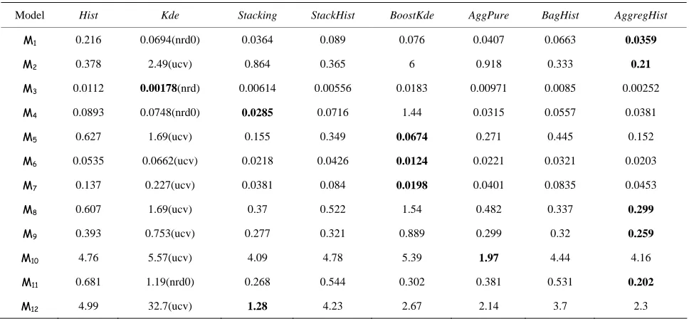
Table 5. 100 × MISE with n = 1000 and M = 200.
M
M1 0.216 0.0694(nrd0) 0.0364 0.089 0.076 0.0407 0.0663 0.0359
M2 0.378 2.49(uc 0.864 0.3 6 8 0.333 21
M3 0.0112 0.00178( 0.00614 0.00 0.0183 71 0.0085 2
M4 0.0893 0.0748(nr 0.0285 0.07 1.44 5 0.0557
M5 0.627 1.69(ucv) 0.155 0.349 0.0674 0.445 152
M6 0.0535 0.0662(u 0.0218 0.04 0.0124 1 0.0321 .0203
M7 0.137 0.227(uc 0.0381 0.0 0.0198 1 0.0835
M8 0.607 1.69(uc 0.37 0.5 1.54 2 0.337 299
M9 0.393 0.753(uc 0.277 0.3 0.889 9 0.32 259
M10 4.76 5.57(uc 4.09 4.7 5.39 4.44 4.16
M11 0.681 1.19(nrd 0.268 0.5 0.302 1 0.531 202
M12 4.99 32.7(ucv) 1.28 4.23 2.67 2.14 3.7 2.3
v) 65 0.91 0.
nrd) 556 0.009 0.0025
d0) 16 0.031 0.0381
0.271 0.
cv) 26 0.022 0
v) 84 0.040 0.0453
v) 22 0.48 0.
v) 21 0.29 0.
v) 8 1.97
0) 44 0.38 0.
w rea he samp ze. Ense ethod timators outperform largely the Hist and Kde in most cases except e mod ard ga ,
hen inc sing t le si mble m s es-
thre els (stand ussian 102
ly the and student distributions) for n = 100, and on 102
model for n 0 an r the n
mo Boo give result the lar
valu of n and acking s
othe gorith he st nd the t ular dist but for 00. F M10, A e achie the perfo nce. F aining ation m els, egH utperf the othe thods wh
n = 0. W it is d ieve th est erro is still very c to the cially f most ch leng distri ns used s M8 to .
5. Conclusion
In this paper we have given a brie
existing approaches for density estimation based on ag-
gr shown a wide sim
tion at, lik super g, en method
giv e to density rs than ra
and Ker ty Among t xistin
me s we teste tensio stacki
(Sta g)an oostin ) as w the mo recent approa und in ure call ure.
W ve a ggest w alg s amo
whi wo o Bag reg mbine
larg mber istogram t random the data usin str ples w ggregH the or gin ata s domizi istogra akpoint
AggregHist gi very go s for mo the situ
tion pecia r large izes, an s easy implement and has the lowest computation cost among
all t ble d tima
Most of the presented algorithms may be extended to the m riate ca are no der stud em- pirically and theor ly. All imulation d the
meth ve bee ement thin an age
availa pon requ
6. Acknowledgements
The a would o than de Denia d Ri- cardo an for useful ons an gges- tions t ve impro this work
REFERENCES
[1] L. Breiman, “Ba Predicto achine Le , Vol. 24, No. 2, 1996, pp. 123-140.
0.1007/BF00058655 = 50 d 1000. Fo gaussia
he ensem ensity es tors.
ultiva se and w un y both etical the s s an ods ha n impl ed wi R pack
ble u est.
uthors like t k Clau u an
Fraim many discussi d su
hat ha ved .
gging rs,” M arning
mixtures dels stKde s the best s for gest
es (500 ms for t
1000). St
udent a outperform riang the ri- r al
ions n = 10 or model ggPur ves best rma or the rem simul od-
Aggr ist o orms all r me en 100 hen oesn’t ach e low r, it
lose best espe or the
M
al-ing butio in model 12
f summary of most http://dx.doi.org/1
[2] Y. Freund and R. E. Schapire, “A Decision-Theoretic Ge-
n of Le nd A to
Boosting,” Jou ystem ces,
V .
119-http://dx.doi.org/10.1006/jcss.1997.1504
neralizatio On-Line arning a pplication
rnal of Computer and S
997, pp
Scien
ol. 55, No. 1, 1 139.
egation. We have using range of ula- s th e for vised learnin semble s e ris better estimato the Histog m
the thod
nel Densi have
Estimators. d direct ex
he e ns of
g ng
ckin d of b g (BoostKde ell as st ch fo the literat ed AggP
e ha lso su ed three ne orithm ng ch t f them Hist and Agg Hist co a e nu
g boot of h ap sam
s. BagHis
hereas A
izes
ist uses i- al d et, ran ng the h m bre s.
ves od result st of a- s es lly fo sample s d it i to
[3] L an, “Sta gress chine L ol.
24, No. 1, 1996, 64.
[4] L an, “Ra Forests hine Lea ol.
45, No. 1, 2001, pp. 5-32.
h .doi.org 3/A:10 04324
. Breim cked Re ion,” Ma earning, V pp.
49-. Breim ndom ,” Mac rning, V
ttp://dx /10.102 109334
[5] P and D lpert, “Linearly Combining Den- sit mators v king,” e Learni l. 36, N p. 59-83
[6] M. Jones, O. Linton J. Nielse mpl s Re-
du for Density Es Biom , Vol.
82, No. 2, 1995, pp. 327-338.
http://dx.doi.org/10.1093/biomet/82.2.327 . Smyth . H. Wo
y Esti ia Stac Machin ng, Vo
o. 1, p .
and n, “A Si
timation,”
e Bia
etrika
[13] J. S. Marron and P. Wan Mean rated
e Annals of Statistics, Vol. 20, No. 2, .
oi.or /aos 653
[7] e “Lookin mps: Boosting and Ba
Density Estimation,” Com Data Analysis, Vol. 38, No. 4, 200
//dx rg/10.1016 7-9473(0 4 G. Ridg
ging for
way, g for Lu g-
putational Statistics &
2, pp. 379-392. http: .doi.o /S016 1)00066-[8] Rosse Segal, “Boosting Densit mation,”
vance ural rocess ems, V
002, p 8.
[9] sting for
ussia res,” atio ing, V
16, 2
508-40-30499-9_78 S.
Ad
t and E.
s in Ne
y Esti
ing Syst ol.
Information P
15, MIT Press, 2 p. 641-64
X. Song, K. Yang and M. Pa Ga
vel, “Density
Neural Inform
Boo
n Process ol. n Mixtu
33
http://dx.doi.org/10.1007/978-3-5 004, pp. 515.
[10] H. W “Stacke ization,” l Networ
, No. 2, 1992, p
D. olpert, d General Neura ks,
Vol. 5
http://dx.doi.org/10.1016/S0893-6080(05)80023-1 p. 241-259.
[11] Rigol A. B. “Linear nvex A
gatio ensity E ,” Mathe l Metho of Statistics, Vo. 16, No. 3, 2007, pp. 260-280.
p://dx g/10.3 307070
P. let and Tsybakov, and Co g-
gre n of D stimators matica ds
htt .doi.or 103/S10665 30052
M. d, “Exact Integ Square Error,” Th
2004, pp. 712-736
http://dx.d g/10.1214 /1176348
[14] B. lverman, nsity E on for St nd
Data Analysis,” an and ondon,
[15] A. Bowman, “An Alternative n
for th Estimates,” Biometr .
71, No. 2, 1984 360.
http://dx.doi.org/ 3/biom .353
W. Si “De
Chapm
stimati Hall, L
atistics a 1986.
Method of Cross-Validatio e Smoothing of Density
pp.
353-ika, Vol
10.109 et/71.2
[16] S ther, “ ty Estim Statistica ce,
V No. 4, 2 .
588-h doi.org 4/0883 000002 . J. Shea
ol. 19,
Densi 004, pp
ation,” 597.
l Scien
ttp://dx. /10.121 423040 97
[17] W e, M. M . Sper A. We on-
p ic and metr ls,” Spr rlag,
Heidelberg, 2004
http://dx.doi.org/10.1007/978-3-642-17146-8 . Härdl
arametr
üller, S Semipara
lich and ic Mode
rwatz, “N inger Ve .
[12] Di M and C. , “Boosting Kernel De sity Estimates: A Bias Reduction Technique?” Biometrika,
l. 91, No. 1, 2004,
10.1093/biomet/91.1.226
M. arzio C. Taylor n-
Vo pp. 226-233.
http://dx.doi.org/
[18] S ther an Jone Reliable ased
Bandwidth Selec Method Density E tion,”
Journal of the Royal Statistical Society, Vol. 53, No. 3, 1991, pp. 683-69
. J. Shea d M. C. s, “A Data-B
tion for stima
0.
Appendix
Different Choices for the Ban KDE
dwidth Selection in
If T
x1,,xn
denotes a sample obtained from a ran-dom variable X with density f, the kernel density estima- tion of f at point x is:
1
1
ˆ n i
h
i
x x
f x K
nh h
(11)where K is a kernel function.
A usual measure of the difference of the estimate den- sity and the true density is the Mean integrated Sq Error (MISE) which may be written as:
uared
2ˆ Bias ˆ
ˆ h h
Va dr h d
MISE f f x x
f x x
It is well known
(12)
4 2 1 ˆ h 2 4 4 1 hMISE f R K K R f nh
o o h
nh
ith and where
w h0 nh R g
g2
x dxnd
a 2
K
x K x2
dxed Squared Error (AMI
The Asymptotic Mean Inte-
rat SE) is:
g
4 2
2 1 ˆ 4 h h
AMISE f R K K R f
nh
(13)
nd it is minimized for a
1 5 * 1 2 2 R K h nK R f
5 (14)
Taking Gaussian kernel K and assuming that the un- erlying distribution is normal, Silverman ([14]) showed
at the expression of is d
th h*
1 5
ˆ 1.06 min ,IQR
h n 1.34
NRD
where ˆ
(15)
and IQR are the standard deviation and the interquantile distance respectively of the sample. This is known as Silverman’s rule of thumbs. Furthermore Sil- verman recommended to use for the constant the values 0.9 (Nrd0) or 1.06 (Nrd).
Another choice of the bandwidth is given by the cross validation method ([15]). Here we consider the Integrated squared error (ISE) which is given by
ˆ ˆ2 ˆ 22
h h h
ISE f
f
f f
f (16)Observe that the last term does not involve h. The least squares cross-validation is
2
1
2 n
h h i
i
LCSV h f f x
n
ˆ
ˆi(17)
where fˆh i
denotes the kernel estimator constructed from the data without the observation i. In [17], it is prov- ed rewriting
2 2 1 1 1ˆ d n n j i
h
i j
x x
f x x K K
h n h
(18)where * denotes the convolution, that LSCV h
is an estimator of ISE f
ˆh
f2.
Moreover it is easy to veri-
fy that
CSV h
MIS
ˆ 2
d
h
E L E f
f x x, thus theleast squares cross-validation is also called unbiased cross- validation. We denote by the value of h which mi- nimizes
ucv
h
LSCV h . , the plug
Finally -in me of Sheather and Jones re- places the unknown
thod
R f used in the optimal value of
h by an estimator R f