Experimental Investigation and Optimization of Process Parameters in Abrasive Water Jet Machine

(1)

EXPERIMENTAL INVESTIGATION AND OPTIMIZATION OF PROCESS

PARAMETERS IN ABRASIVE WATER JET MACHINE

M. SAGAR

Final Year B.Tech, Mechanical Engineering, St.Martin’s Engineering College, Secunderabad, Telangana, India

---*---Abstract -**

Here accommodating a non-conventional

machining process in which mechanical energy of water along with abrasives is used for removing material. This process is observed in Abrasive Water Jet Machining. For this, Design of Experiments are selected and optimized by adopting Taguchi technique.

Taguchi method is a statistical method developed by Taguchi and Konishi. Initially it was developed for improving the quality of goods manufactured (manufacturing process development), later its application was expanded to many other fields in Engineering, such as Biotechnology etc. Professional statisticians have acknowledged Taguchi’s efforts especially in the development of designs for studying variation. Success in achieving the desired results involves a careful selection of process parameters and bifurcating them into control and noise factors. Selection of control factors must be made such that it nullifies the effect of noise factors.

Taguchi Method involves identification of proper control factors to obtain the optimum results of the process. Orthogonal Arrays (OA) are used to conduct a set of experiments. Results of these experiments are used to analyse the data and predict the quality of components produced.

The AWJM process parameters selected are Abrasive Flow Rate, thickness of the material, Pressure, Nozzle Diameter, Stand of Distance, Time & Kerf Factors. This process will become a greater advantage in machining industry.

Key Words: Abrasive Flow Rate (g/min), Stand of Distance (mm), Nozzle Diameter (mm), Pressure, Material Removal Rate (mm3 /min), Silicon Carbide, Signal to Noise Ratio, Analysis Of Variance, Design of Experiments, Width of Cut.

1. INTRODUCTION

Abrasive water jet cutting is an extended version of water jet cutting; in which the water jet contains abrasive particles such as silicon carbide or aluminum oxide in order to increase the material removal rate above that of water jet machining. Almost many type of material ranging from hard brittle materials such as ceramics, metals and glass to extremely soft materials such as foam and rubbers can be cut by abrasive water jet cutting. The narrow cutting stream and computer controlled movement enables this process to produce parts accurately and efficiently. This machining process is especially ideal for cutting materials that cannot be cut by laser or thermal cut. Metallic, non-metallic and advanced composite materials of various thicknesses can be

cut by this process. This process is particularly suitable for heat sensitive materials that cannot be machined by processes that produce heat while machining.

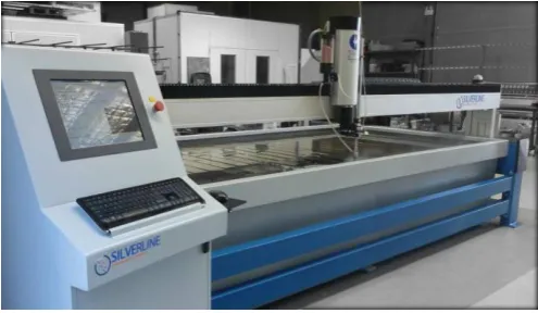
[image:1.595.308.556.324.468.2]

The schematic of abrasive water jet cutting is shown in Figure 1. This is similar to water jet cutting apart from some more features underneath the jewel; namely abrasive, guard and mixing tube. In this process, high velocity water exiting the jewel creates a vacuum which sucks abrasive from the abrasive line, which mixes with the water in the mixing tube to form a high velocity beam of abrasives.

Fig -1: Abrasive Water jet Machine

1.1 Applications

Abrasive water jet cutting is highly used in aerospace, automotive and electronics industries. In aerospace industries, parts such as titanium bodies for military aircrafts, engine components (aluminum, titanium, and heat resistant alloys), aluminum body parts and interior cabin parts are made using abrasive water jet cutting.

In automotive industries, parts like interior trim (head liners, trunk liners, and door panels) and Fiber glass body components and bumpers are made by this process. Similarly, in electronics industries, circuit boards and cable stripping are made by abrasive water jet cutting.

1.2 Advantages of abrasive water jet cutting

 In most of the cases, no secondary finishing required

 No cutter induced distortion

 Low cutting forces on work pieces

 Limited tooling requirements

(2)

 Smaller kerf size reduces material wastages

 No heat affected zone

 No cutter induced metal contamination

 Eliminates thermal distortion

 No slag or cutting dross

 Precise, multi plane cutting of contours, shapes, and bevels of any angle.

1.3 Limitations of abrasive water jet cutting

● Cannot drill flat bottom

● Cannot cut materials that degrades quickly with moisture

● Surface finish degrades at higher cut speeds which are frequently used for rough cuts

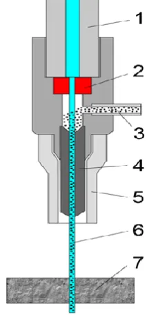
[image:2.595.105.212.355.584.2]

The major disadvantages of abrasive water jet cutting are high capital cost and high noise levels during operation.

Fig -2: SCHEMATIC DIAGRAM 1. High pressure tube

2. Orifice (sapphire) 3. Abrasive

4. Nozzle / mixing chamber 5. Guard

6. High pressure stream 7. Material to be cut

1.4 PARAMETERS

● PRESSURE

● METAL REMOVAL RATE (MRR)

● STAND OF DISTANCE (SOD)

1.5 EFFECTS OF PARAMETERS:-

1.5.1 EFFECT OF ABRASIVE FLOW RATE ON DEPTH OF CUT

The effect of abrasive flow rate (ma) on depth of cut was tested. The tests were conducted at different abrasive flow rates. Abrasive flow rate found that the increase of abrasive flow rate increases the depth of cut. The general trend of this relation is a polynomial function with high regression ratio R2.

1.5.2 EFFECT OF STAND-OFF DISTANCE ON DEPTH OF CUT

The effect of stand-off distance on depth of cut was tested. The test was conducted at three different stand-off distances and repeated at three abrasive flow rate values. The depth of cut values change barely with the increase of the standoff distance. Therefore, it is concluded that the stand-off distance has no effect on depth of cut in the range of the tests.

1.5.3 EFFECT OF PRESSURE ON MRR

The effect of jet pressure on MMR was tested in range of pressures from 1200 to 3600 Kg/Cm2_{. In this range it was}

found that when the jet pressure increased the MRR was almost of a fixed value. The tests were repeated at two abrasive flow rates. Therefore, it is concluded that jet pressure has no effect on MMR in the test range.

2. LITERATURE REVIEW

1. D.V.Srikanth and M. Srinivasa Rao [1] Explained the effect of abrasive mass flow rate on the MRR in AWJM. It was concluded that SOD increases the MRR and depth rate increase and on attaining optimal value it begins decreasing.

2. B. Sidda Reddy at al. [2] Investigated optimization of the input parameters of abrasive water jet machining process by means of Taguchi method. The use of Analysis of Variance (ANOVA) and signal to noise ratio (S/N) ratio to optimize different parameters for obtaining efficient Material Removal Rate (MRR) and surface roughness.

(3)

3. EXPERIMENTAL INVESTIGATION

3.1 INTRODUCTION

Glass specimen of 10mm thickness is used. Abrasive type is used is Sic (silicon carbide intensifier pumping system has operating pressure of up to 380 MPa.) The motion of the nozzle is controlled by a computer. The principle AWJM is, abrasives like aluminium oxide, are fed into the nozzle via an abrasive inlet the high pressure. Water jet metal cutting machine yields vary little heat and therefore there is no heat affected zone (HAZ).Water jet machining is also considered as “cold cut” process and therefore is safe for cutting flammable materials such as plastic and polymers.

3.2 THE EXPERIMENTATION

The machine is equipped with a gravity feed type of abrasive hopper, an abrasive feeder system, a pneumatically controlled valve and a work piece table. A sapphire or if ice was used to transform the high-pressure water into a Collimated jet, with a tungsten carbide nozzle of 2mm diameter to form an abrasive water jet. The abrasives used were 60 mesh garnet particles. The abrasives were delivered using compressed air from a hopper to the mixing chamber and were regulated. The abrasive water jet pressure is manually controlled using the pressure gauge. The standoff distance 1.5,2.5 and 3.5. The traverse speed was controlled automatically by the abrasive waterjet system programmed by NC code.

3.3 PROCEDURE

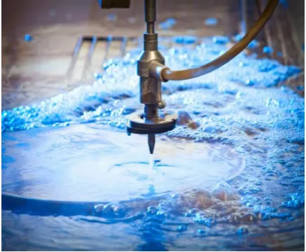
[image:3.595.314.558.79.221.2]

To achieve a thorough cut it was required that the combination of the process variables give the jet enough energy to penetrate through the specimens. The variables in AWJM were varied and readings were taken with combination of process parameters together the required data. Three different readings were taken at each sample and the average readings were calculated.

[image:3.595.324.546.256.399.2]

Fig -3: Machining Operation 1

Fig -4: Machining Operation 2

Fig -5: Final Work Piece

4. OPTIMISATION USING TAGUCHI & ANOVA

TAGUCHI

Taguchi has envisaged a new method of conducting the design of experiments which are based on well defined guidelines. This method uses a special set of arrays called orthogonal arrays. These standard arrays stipulate the way of conducting the minimal number of experiments which could give the full information of all the factors that affect the performance parameter. The crux of the orthogonal arrays method lies in choosing the level combinations of the input design variables for each experiment

.

ANOVA

Analysis of Variance (ANOVA) is a statistical method used to test differences between two or more means. It may seem odd that the technique is called "Analysis of Variance" rather than "Analysis of Means." As you will see, the name is appropriate because inferences about means are made by analyzing variance.

[image:3.595.52.271.563.743.2]

(4)

Pairwise Comparisons among Means" showed how to test differences among means.

5. Taguchi Design

Design Summary Taguchi Array L9(3^3)

Factors 3

Runs 9

Columns of L9 (3^4) array: 1 2 3

Factors Levels

Pressure 1200,2400,3600 AFR 100,200,300 SOD 1.5,2.5,3.5 Taguchi Analysis: MRR versus PRESSURE, AFR, SOD

Response Table for Signal to Noise Ratios Larger is better

Level PRESSURE AFR SOD 1 11.44 15.44 17.05 2 16.80 15.66 16.52 3 21.15 18.29 15.82 Delta 9.71 2.85 1.23

Rank 1 2 3

Response Table for Means

Level PRESSURE AFR SOD 1 4.020 6.817 7.533 2 7.923 6.407 9.993 3 13.303 12.023 7.720 Delta 9.283 5.617 2.460

Rank 1 2 3

Taguchi Analysis: KERF versus PRESSURE, AFR, SOD Response Table for Signal to Noise Ratios

Smaller is better

Level PRESSURE AFR SOD

1 16.82 16.82 15.99

2 16.82 17.65 16.82

3 16.82 15.99 17.65

Delta 0.00 1.67 1.67

Rank 3 1 2

Response Table for Means

Level PRESSURE AFR SOD

1 0.1500 0.1500 0.1667 2 0.1500 0.1333 0.1500 3 0.1500 0.1667 0.1333 Delta 0.0000 0.0333 0.0333

Rank 3 1.5 1.5

General Linear Model: MRR versus PRESSURE, AFR, SOD Method

Factor coding (-1, 0, +1) Factor Information

Factor Type Levels Values

PRESSURE Fixed 3 1200, 2400, 3600 AFR Fixed 3 100, 200, 300 SOD Fixed 3 1.5, 2.5, 3.5

Analysis of Variance

Source DF Adj SS Adj MS Value F- Value

P-PRESSURE 2 130.36 65.180 1.09 0.479 AFR 2 58.82 29.412 0.49 0.671 SOD 2 11.25 5.627 0.09 0.914 Error 2 120.01 60.006

Total 8 320.45

Model Summary

S R-sq R-sq(adj) R-sq(pred) 7.74635 90.55% 0.00% 0.00%

Coefficients

Term Coef Coef SE Value T- Value P- VIF

Constant 8.42 2.58 3.26 0.083 PRESSURE

1200 -4.40 3.65 -1.20 0.352 1.33 2400 -0.49 3.65 -0.13 0.905 1.33

AFR

100 -1.60 3.65 -0.44 0.704 1.33 200 -2.01 3.65 -0.55 0.637 1.33

SOD

(5)

M R R

= 8.42 4.40 PRESSURE_1200

0.49 PRESSURE_2400 + 4.89 PRESSURE_3600 1.60 AFR_100

- 2.01 AFR_200 + 3.61 AFR_300 - 0.88 SOD_1.5 + 1.58 SOD_2.5 - 0.70 SOD_3.5

General Linear Model: KERF versus PRESSURE, AFR, SOD Method

Factor coding (-1, 0, +1) Factor Information

Factor Type Levels Values

PRESSURE Fixed 3 1200, 2400, 3600 AFR Fixed 3 100, 200, 300 SOD Fixed 3 1.5, 2.5, 3.5

Analysis of Variance

Source DF Adj SS Adj MS Value F- Value P-PRESSURE 2 0.000000 0.000000 0.00 1.000 AFR 2 0.001667 0.000833 0.14 0.875 SOD 2 0.001667 0.000833 0.14 0.875 Error 2 0.011667 0.005833

Total 8 0.015000

Model Summary

S R-sq R-sq(adj) R-sq(pred) 0.0763763 84.22% 0.00% 0.00%

Coefficients

Term Coef SE Coef T-Value Value P- VIF

Constant 0.1500 0.0255 5.89 0.028

PRESSURE

1200 -0.0000 0.0360 -0.00 1.000 1.33

2400 -0.0000 0.0360 -0.00 1.000 1.33

AFR

100 -0.0000 0.0360 -0.00 1.000 1.33

200 -0.0167 0.0360 -0.46 0.689 1.33

SOD

1.5 0.0167 0.0360 0.46 0.689 1.33

2.5 0.0000 0.0360 0.00 1.000 1.33

Regression Equation

K E R F

0.1500 0.0000 PRESSURE_1200

0.0000 PRESSURE_2400 + 0.0000 PRESSURE_3600 - 0.0000 AFR_100 - 0.0167 AFR_200 + 0.0167 AFR_300 + 0.0167 SOD_1.5

+ 0.0000 SOD_2.5 - 0.0167 SOD_3.5 Response Optimization: KERF, MRR

Parameters Respo

nse Goal wer Lo Target per Up Weight Importance KERF Minimum 0.1 0.2 1 1

MRR Maximum 2.17 22.6 1 1

Solution

Soluti

on PRESSURE AFR SOD KERF Fit MRR Fit

Compos ite Desirab

ility 1 3600 200 2.5 0.133

333 12.8722 0.590959

Multiple Response Prediction

Variable Setting

PRESSURE 3600

AFR 200

SOD 2.5

Respon

se Fit Fit SE 95% CI 95% PI

KERF 0.1333 0.06

74 (-0.1565, 0.4231) (-0.3048, 0.5715) MRR 12.87 6.83 (-16.52,

42.27) (-31.57, 57.31)

PRES

SURE AFR SOD KERF MRR SNRA1 MEAN1 SNRA2 MEAN2

1200 100 1.5 0.20 5.6

5 15.0410 5.65 13.9794 0.20

1200 200 2.5 0.15 4.2

4 12.5473 4.24 16.4782 0.15

1200 300 3.5 0.10 2.1

7 6.7292 2.17 20.0000 0.10

2400 100 2.5 0.10 3.1

4 9.9386 3.14 20.0000 0.10

2400 200 3.5 0.15 9.3

3 19.39

76

9.33 16.4

(6)

2400 300 1.5 0.20 11.

30 21.0616 11.30 13.9794 0.20

3600 100 3.5 0.15 11.

66 21.3340 11.66 16.4782 0.15

3600 200 1.5 0.10 5.6

5 15.0410 5.65 20.0000 0.10

3600 300 2.5 0.20 22.

60 27.0822 22.60 13.9794 0.20

6. CONCLUSION

The present study is limited to specific materials of certain thickness, whose hardness is well known. The optimization techniques are also for those particular combinations. It is considered worthwhile exercise to arrive at generalized parameters for a particular group of materials, which can be classified using the Brinells /Rockwell hardness values or such common parameters. For arriving of such a generalized equation more experiments need to be performed for different varieties of material. Abrasive materials are used as a tool in these cases is also a much needed subject of study. As advances in materials technology is progressing fast we may have to substitute the present abrasive particles which have less erosion rate in nozzles, but high machining rate at the work piece. The use of Nano materials may be an answer to this improvement in this technology.

Researches towards specific industrial application may result in better usage of the AWJM process for commercial exploitation.

ACKNOWLEDGEMENT

I express my sincere gratitude to Prof. D V Srikanth, Head, Dept. of Mechanical Engineering, SMEC, Secunderabad, for his stimulating guidance, continuous encouragement and supervision throughout the course of present work.

I am extremely thankful to Dr. P. Santosh Kumar Patra, Principal, SMEC, for providing me infrastructural facilities to work in, without which this work would not have been possible.

REFERENCES

1. M. Hashish, A model for abrasive water jet machining, J. Engg. Materials Tech., Vol.111, (1989), pp.154-162.

2. Module 9, lesson 37, non-conventional machining, version 2 ME, IIT Kharagpur.

3. Effects of Process Parameters on Depth of Cut in Abrasive Waterjet Cutting of Cast Iron by M.Chithirai Pon Selvan, Dr.N.Mohana Sundara Raju, Dr.R.Rajavel.

Experimental Investigation and Optimization of Process Parameters in Abrasive Water Jet Machine