On Rotational Robustness of Shapiro Wilk Type Tests for Multivariate Normality

http://dx.doi.org/10.4236/ojs.2014.411090

On Rotational Robustness of Shapiro-Wilk

Type Tests for Multivariate Normality

Richie Lee, Meng Qian, Yongzhao Shao

Division of Biostatistics, New York University School of Medicine, New York, USA Email: [email protected]

Received 14 October 2014; revised 10 November 2014; accepted 16 November 2014

Copyright © 2014 by authors and Scientific Research Publishing Inc.

This work is licensed under the Creative Commons Attribution International License (CC BY). http://creativecommons.org/licenses/by/4.0/

Abstract

The Shapiro-Wilk test (SWT) for normality is well known for its competitive power against nu-merous one-dimensional alternatives. Several extensions of the SWT to multi-dimensions have also been proposed. This paper investigates the relative strength and rotational robustness of some SWT-based normality tests. In particular, the Royston’s H-test and the SWT-based test pro-posed by Villaseñor-Alva and González-Estrada have R packages available for testing multivariate normality; thus they are user friendly but lack of rotational robustness compared to the test pro-posed by Fattorini. Numerical power comparison is provided for illustration along with some practical guidelines on the choice of these SWT-type tests in practice.

Keywords

Multivariate Normality, R Packages, Robust Power, Shapiro-Wilk Test, Rotational Robustness

1. Introduction

Normal distributions are of central importance in statistical inference and in numerous applications. Thus, test-ing for normality includtest-ing assesstest-ing multivariate normality has been studied extensively in statistics. For in-stance, in a research monograph, Thode [1] reviewed more than 30 formal statistical procedures proposed spe-cifically for testing normality. For univariate data, the Shapiro-Wilk test (SWT) [2] for normality is the well- known benchmark of omnibus tests in terms of competitive power performance against a broad range of alterna-tives. Many extensions of the univariate SWT to multi-dimensions have been developed [1], and at least two R packages for testing multivariate normality have recently been made based on the SWT-based tests by Royston

insights and guidelines on when to use them would be of practical interest. This paper discusses the relative strength and rotational robustness of these user-friendly SWT-based tests and provides some guidelines for se-lecting tests in practical applications. In the next section we briefly review the original SWT [2] and two SWT-based tests for multivariate normality with R packages [3]-[9]. Section 3 discusses rotational robustness and the FA test [10]. Section 4 discusses the Iris data example and reports Monte Carlo simulation results. Sec-tion 5 provides some guidelines and remarks. The R code for the FA test is provided in the appendix.

2. The SWT-Based Normality Tests with R-Packages

Originally created to test univariate distributions for normality, given univariate data X =

(

x1,,xn

)

, the

Sha-piro-Wilk test (SWT) [2] statistic is

( )

(

)

(

)

2 1 2 1 n i i i X _n i n i a x W x X = = = −

∑

∑

where x_{( )1},,x_{( )n} are the order statistics of the univariate data X =

(

x₁,,x_n

)

, X_n is the sample mean, and

the constants

{ }

a_i are

(

)

(

T 1 1

)

1 2 T 1 1, , n

a  a = m V V m− − − m V− , with m=

(

m₁,,m_n

)

T and

V

being the mean vector and covariance matrix of the order statistics of a random standard normal sample of size n. The univa-riate SWT can be performed easily in R using the function shapiro.test based on Royston’s algorithms [3] [4]. The Shapiro-Wilk test (SWT) for normality is well known for its competitive power against numerous one-di- mensional alternatives. Many extensions of the SWT to the multivariate case have been proposed in the litera-ture including Royston’s H-test [3]-[7] and a new multivariate extension of the SWT by Villaseñor-Alva and González-Estrada [8]. The first step in the extension of SWT proposed in [8] is to standardize the multiva-

riate data X =

(

X₁,,Xp

)

T by substracting the sample mean Xn and multiplying by the square root of the

inverse of its covariance matrix S_n. It is known that the covariance matrix S_n of a

p

-variate normal is non-

degenerate with probability one. Without loss of generality, let

1 2

n

S− be the symmetric square root of S_n−1 and

denote the standardized data as

(

)

1

2 _{– , 1, , ,}

n n

S− X i n

= =

i i

Z X  and Z =

(

Z1,,Zn

)

is the

p n

×

data matrix.

Under the null hypothesis, X has a multivariate normal distribution and Z has approximately the multiva-riate standard normal distribution [8]. Villaseñor-Alva and González-Estrada [8] proposed to use the following test statistic

( )

* 1 1 i p C i W W p = =

∑

Z where i C

W is the univariate SWT statistic evaluated on the ith coordinate of the standardized data Z=

(

C1,,Cp

)

T

where C_i =

(

Z_i1,,Z_in

)

T, i=1,,p. This test is easy to understand and has been programmed into an R pack-

3. Rotational Robustness and the FA Test of Fattorini

The multivariate normal distributions have rotational invariance. In particular, X =

(

X X₁, ₂

)

is bivariate

nor-mal if and only if U X

( ) (

= X₁−X₂,X₁+X₂

)

is bivariate normal. In general, X =

(

X X₁, ₂

)

is bivariate

normal if and only if U_θ

( )

X =

(

cos

( )

θ X₁−sin

( )

θ X₂, cos

( )

θ X₁+sin

( )

θ X₂

)

is bivariate normal for any

an-gle

θ

. Also, when X =

(

X X₁, ₂

)

is not bivariate normal, U_θ

( )

X is not bivariate normal for all angle

θ

[15]. When θ =0,U_θ

( )

X =X. Thus if we know when

θ =

0

the data is more non-normal than at other an-gles, we would prefer testing normality for X=

(

X X₁, ₂

)

. Similarly, if we know θ =π 4 is more non-normal than at other angles, we would prefer testing normality for U X

( ) (

= X₁−X₂,X₁+X₂

)

instead of testing nor-mality for X =

(

X X₁, ₂

)

. Ideally, when X is not bivariate normal, we might desire a normality test with good power for detecting non-normality of U_θ

( )

X for all angle

θ

_{or a test that can automatically search for the} most non-normal direction to test, i.e., one might hope to have a robust normality test when there is no clue about which angle corresponds to the most non-normal data. Among the SWT-based test for multivariate nor-mality, the FA test proposed by Fattorini [10] and a similar test proposed by Malkovich and Afifi [12] actually search for the most non-normal direction and thus would be more rotationally robust than either the mvShapi-

roTest or the Royston test. The FA test statistic is given by FA

( )

min

(

_{( )}

)

j

j n≤ WZ θ =

Z , where _{( )}

j

Z

W _θ is the

SWT statistic evaluated at Z_j

( )

θ

=ZT_jZ , where Zj =

(

Z₁j,,Zpj

)

T i.e.

(

)

1 2

n n

S− X

= −

j j

Z X is the jth

standardized observation j=1,,n, and Z=

(

Z1,,Zn

)

is the

p n

×

data matrix. Possibly due to the ro-

bust power properties of the FA test, Thode [1] recommended the FA test as a generally powerful multivariate normality test besides the HZ test by Henze and Zirkler [11] after reviewing more than 30 tests for normality in-cluding both SWT-based and non-SWT based tests. The HZ test uses empirical characteristic functions instead of using extensions of the SWT.

4. The Iris Data Example and Numerical Studies

4.1. The Iris Data Example

The Iris data set is a well-known multivariate data set collected to measure the morphologic variation of Iris flowers of three related species. The data set consists of 50 samples from each of three species of Iris including setosa, virginica and versicolor. For each sample, four variables were measured including the length and the width of the sepals and petals, in centimeters. Fisher [16] used the Iris data to demonstrate the use of unclassi-fied observations in estimating discriminant function. The non-normality of the multivariate Iris data has been investigated by many statisticians [17] [18]. For illustration, we consider the bivariate normality of the Iris data set by using the length and the width of the sepals of two of the species Iris setosa,and Iris versicolor that are the first two columns and first 100 rows of the Iris data. The p-values of the mvShapiro.Test and royston.test in R were 0.26 and 0.37, respectively. Thus both tests fail to detect non-normality when testing X. However, if we test U(X) instead of X for normality, both the mvShapiro.Test and royston.test have very small p-values, 0.0003 and 0.0018, respectively, providing significant evidence of non-normality. Thus in this case, the two tests based on testing U(X) are more powerful than testing X. For the above data the FA test has p-values < 0.001 in testing both X and U(X) indicating rotational robustness.

4.2. Simulation Studies

that exceeded the previously calculated critical values under 50,000 samples from each alternative. Similarly the royston package in R is used to calculate critical values of the royston.test based on 500,000 samples from the standard bivariate normal distribution and the empirical power based on 50,000 samples from each alternative distribution. Using the same set up, the critical values and power of the FA test [10] were obtained using the R code provided in the Appendix. Note that all three tests are applied to standardized data in our simulations to make sure Type I errors are correct under multivariate normality with unknown mean vector and covariance ma-trix and to ensure fair power comparison.

4.3. Simulation Findings

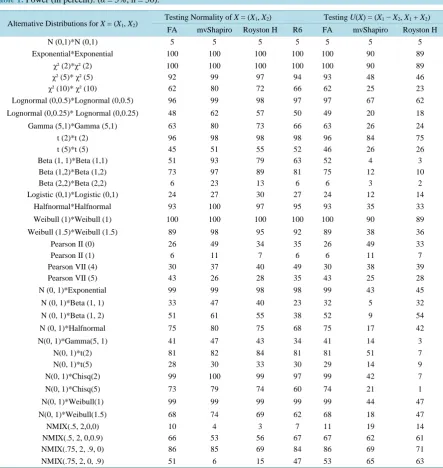
[image:4.595.94.538.243.712.2]

The simulated power is illustrated in Table 1for the sample size n = 50 and θ =0 orπ 4. The power patterns are the same for other sample sizes e.g. n = 25 or 100, thus not presented. More specifically, in Table 1, the al-

Table 1.Power (in percent): (α = 5%, n = 50).

Alternative Distributions for X = (X1, X2)

Testing Normality of X = (X1, X2) Testing U(X) = (X1 − X2, X1 + X2)

FA mvShapiro Royston H R6 FA mvShapiro Royston H

N (0,1)*N (0,1) 5 5 5 5 5 5 5

Exponential*Exponential 100 100 100 100 100 90 89

χ² (2)*χ² (2) 100 100 100 100 100 90 89

χ² (5)* χ² (5) 92 99 97 94 93 48 46

χ² (10)* χ² (10) 62 80 72 66 62 25 23

Lognormal (0,0.5)*Lognormal (0,0.5) 96 99 98 97 97 67 62

Lognormal (0,0.25)* Lognormal (0,0.25) 48 62 57 50 49 20 18

Gamma (5,1)*Gamma (5,1) 63 80 73 66 63 26 24

t (2)*t (2) 96 98 98 98 96 84 75

t (5)*t (5) 45 51 55 52 46 26 26

Beta (1, 1)*Beta (1,1) 51 93 79 63 52 4 3

Beta (1,2)*Beta (1,2) 73 97 89 81 75 12 10

Beta (2,2)*Beta (2,2) 6 23 13 6 6 3 2

Logistic (0,1)*Logistic (0,1) 24 27 30 27 24 12 14

Halfnormal*Halfnormal 93 100 97 95 93 35 33

Weibull (1)*Weibull (1) 100 100 100 100 100 90 89

Weibull (1.5)*Weibull (1.5) 89 98 95 92 89 38 36

Pearson II (0) 26 49 34 35 26 49 33

Pearson II (1) 6 11 7 6 6 11 7

Pearson VII (4) 30 37 40 49 30 38 39

Pearson VII (5) 43 26 28 35 43 25 28

N (0, 1)*Exponential 99 99 98 98 99 43 45

N (0, 1)*Beta (1, 1) 33 47 40 23 32 5 32

N (0, 1)*Beta (1, 2) 51 61 55 38 52 9 54

N (0, 1)*Halfnormal 75 80 75 68 75 17 42

N(0, 1)*Gamma(5, 1) 41 47 43 34 41 14 3

N(0, 1)*t(2) 81 82 84 81 81 51 7

N(0, 1)*t(5) 28 30 33 30 29 14 9

N(0, 1)*Chisq(2) 99 100 99 97 99 42 7

N(0, 1)*Chisq(5) 73 79 74 60 74 21 1

N(0, 1)*Weibull(1) 99 99 99 99 99 44 47

N(0, 1)*Weibull(1.5) 68 74 69 62 68 18 47

NMIX(.5, 2,0,0) 10 4 3 7 11 19 14

NMIX(.5, 2, 0,0.9) 66 53 56 67 67 62 61

NMIX(.75, 2, .9, 0) 86 85 69 84 86 69 71

ternative χ2(5)*χ2(5) stands for a bivariate distribution with the two independent marginal distributions each be-ing the χ2(5) distribution. U_θ

( )

X =

(

cos

( )

θ X₁−sin

( )

θ X₂, cos

( )

θ X₁+sin

( )

θ X₂

)

is non-normal for any given angle when X=

(

X X₁, ₂

)

is from χ2(5)*χ2(5) [15]. However, it is intuitively clear that X₁+X₂ is closer to normal than either X₁ or X₂ by the central limit theorem. Thus the mvShapiroTest and the Roys-ton test both have high power to detect non-normality of χ2(5)*χ2(5) when testing X =

(

X X₁, ₂

)

, but they only have less than 50% power to detect non-normality of U X

( ) (

= X₁−X₂,X₁+X₂

)

. On the other hand, the power for the FA test stays essentially at the same 92% level because it searches for the most non-normal direc-tions to test. The power patterns for testing other alternatives with independent marginal distribudirec-tions are similar. For illustration of alternatives with non-independent marginals, we use the same Pearson II and VII alternatives and the same normal mixture alternatives as in [8]. When marginal distributions are not independent, the

( ) (

= X1−X2,X1+X2

)

U X can be more non-normal than X=

(

X X₁, ₂

)

, then the mvShapiroTest and the Royston test both can have much higher power to detect non-normality when testing U X

( ) (

= X₁−X₂,X₁+X₂

)

than when testing X=

(

X X₁, ₂

)

. This can be seen clearly from the above Iris data example and from the last normal mixture alternative in Table 1, where the mvShapiroTest and the Royston test have only 6% and 15% power when testing X =

(

X X₁, ₂

)

, respectively. However, both tests have much higher power (more than 60% power) when testing non-normality forU X

( ) (

= X₁−X₂,X₁+X₂

)

. From Table 1, if we know the observed marginal distributions are independent and correspond to the most non-normal directions, the mvShapiro.Test or the royston.test in R is a good choice for testing X =

(

X X₁, ₂

)

because of good power. However, the most non-normal angles are typically unknown in practice. In the absence of such information about alternatives, a rotationally robust test such as the FA test might be more desirable than both Royston’s H-test and the mvSha-piro.Test proposed in [8] and [9].

5. Discussion

If we have prior information that X has independent margins and X itself is the most non-normal configu-ration than any of the U_θ

( )

X , then we can use either the mvShapiro.Test or the royston.test in R to detect non-normality. When there is no such information available, one might prefer to use a rotationally robust test such as the FA test. The FA test has not been incorporated into R packages yet, but it can be coded easily using the shapiro.test function in R (see Appendix). Given its rotationally robust property, it is likely to be included in some R packages in the future. It is also likely that some new robust test possibly more powerful than the FA test might be developed. For example, Table 1 also reports a test based on searching for the most non-normal angle in the Royston test among six fixed angles 0, π π π π 5π, , , ,

12 6 4 3 12

θ

 ₌ 

 

  called the R6 test. Note that the R6

test has equal power whether testing X or U X

( ) (

= X₁−X₂,X₁+X₂

)

and seems to have robust power

comparable to the FA test in the bivariate case. Of course, combining SWT-based tests with other non-SWT type tests (e.g. the kurtosis test [18]-[20]) might also worth consideration in order to obtain generally robust and powerful tests such as the combination test developed in [21].

Acknowledgements

The authors would like to thank Dr. Ming Zhou and Dr. Jiqiang Guo for help with R programming and for con-structive conversations. Y.S.’s research is partially supported by the NYU NIEHS Center Grant P30 ES00260 and the NYU Cancer Center Support Grant 2P30 CA16087.

References

[1] Thode Jr., H.C. (2012) Testing for Normality. Marcel Dekker, Inc., New York.

[2] Shapiro, S.S. and Wilk, M.B. (1965) An Analysis of Variance Test for Normality (Complete Samples). Biometrika, 52, 591-611. http://dx.doi.org/10.1093/biomet/52.3-4.591

[3] Royston, T.P. (1982) An Extension of Shapiro and Wilk W Test for Normality to Large Samples. Applied Statistics, 31, 115-124. http://dx.doi.org/10.2307/2347973

[4] Royston, T.P. (1983) Some Techniques for Assessing Multivarate Normality Based on the Shapiro-Wilk W. Applied Statistics, 32, 121-133. http://dx.doi.org/10.2307/2347291

119. http://dx.doi.org/10.1007/BF01891203

[6] Royston, J.P. (1995) Remark AS R94: A Remark on Algorithm AS 181: The W Test for Normality. Applied Statistics,

44, 547-551. http://dx.doi.org/10.2307/2986146

[7] Korkmaz, S. (2013) Royston’s H Test: Multivariate Normality Test. http://cran.r-project.org/web/packages/royston/index.html

[8] Villaseñor-Alva, J.A. and González-Estrada, G. (2009) A Generalization of Shapiro-Wilk’s Test for Multivariate Nor-mality. Communications in Statistics-Theory and Methods, 38, 1870-1883.

http://dx.doi.org/10.1080/03610920802474465

[9] Gonzalez-Estrada, G. and Villaseñor-Alva, J.A. (2013) Generalized Shapiro-Wilk Test for Multivariate Normality. http://rpackages.ianhowson.com/cran/mvShapiroTest/

[10] Fattorini, L. (1986) Remarks on the Use of the Shapiro-Wilk Statistic for Testing Multivariate Normality. Statistica, 46, 209-217.

[11] Henze, N. and Zirkler, B. (1990) A Class of Invariant Consistent Tests for Multivariate Normality. Communications in Statistics-Theory and Method, 19, 3595-3618. http://dx.doi.org/10.1080/03610929008830400

[12] Malkovich, J.F. and Afifi, A.A. (1973) On Tests for Multivariate Normality. Journal of American Statistical Associa-tion, 68, 713-718. http://dx.doi.org/10.1080/01621459.1973.10481358

[13] Mudholkar, G., Srivastava, D. and Lin, C. (1995) Some p-Variate Adaptations of the Shapiro-Wilk Test of Normality.

Communications in Statistics-Theory and Method, 24, 953-985. http://dx.doi.org/10.1080/03610929508831533 [14] Srivastava, M. and Hui, T. (1987) On Assessing Multivariate Normality Based on Shapiro-Wilk W Statistic. Statistics

and Probability Letters, 5, 15-18. http://dx.doi.org/10.1016/0167-7152(87)90019-8

[15] Shao, Y. and Zhou, M. (2010) A Characterization of Multivariate Normality through Univariate Projections. Journal of Multivariate Analysis, 101, 2637-2640. http://dx.doi.org/10.1016/j.jmva.2010.04.015

[16] Fisher, R.A. (1936) The Use of Multiple Measurements in Taxonomic Problems. Annals of Eugenics, 7, 179-188. http://dx.doi.org/10.1111/j.1469-1809.1936.tb02137.x

[17] Looney, S.W. (1995) How to Use Tests for Univariate Normality to Assess Multivariate Normality. The American Sta-tistician, 49, 64-70.

[18] Small, N. (1980) Marginal Skewness and Kurtosis in Testing Multivariate Normality. Applied Statistics, 29, 85-87. http://dx.doi.org/10.2307/2346414

[19] Mardia, K.V. (1974) Applications of Some Measures of Multivariate Skewness and Kurtosis in Testing Normality and Robustness Studies. Sankhyā: The Indian Journal of Statistics, Series B, 36, 115-128.

[20] Srivastava, M.S. (1984) A Measure of Skewness and Kurtosis and a Graphical Method for Assessing Multivariate Normality. Statistics and Probability Letters, 2, 263-267. http://dx.doi.org/10.1016/0167-7152(84)90062-2

[21] Zhou, M. and Shao, Y. (2014) A Powerful Test for Multivariate Normality. Journal of Applied Statistics, 41, 351-363. http://dx.doi.org/10.1080/02664763.2013.839637

Appendix: The R Code for Calculating the FA Test Statistic

“SW” <- function(X) shapiro.test(X)$statistic

“FA” <- function(X) { X < - as.matrix(X) n < - NROW(X) p < - NCOL(X) mu< - apply(X,2,mean) nSinver< - solve((n-1)*cov(X))

Y < - X%*%t ((X-matrix(rep(mu,n),ncol=p,byrow=TRUE))%*%nSinver) return(min(apply(Y,2,SW)))}