http://dx.doi.org/10.4236/ajibm.2015.52007
How to cite this paper: Choi, J., Park, Y.S. and Park, J.D. (2015) Development of an Aggregate Air Quality Index Using a PCA-Based Method: A Case Study of the US Transportation Sector. American Journal of Industrial and Business Manage-ment, 5, 53-65. http://dx.doi.org/10.4236/ajibm.2015.52007
Development of an Aggregate Air Quality
Index Using a PCA-Based Method: A Case
Study of the US Transportation Sector
Jaesung Choi, Yong Shin Park, Ju Dong Park
*Upper Great Plains Transportation Institute, North Dakota State University, Fargo, ND, USA Email: *[email protected]
Received 23 January 2015; accepted 9 February 2015; published 15 February 2015
Copyright © 2015 by authors and Scientific Research Publishing Inc.
This work is licensed under the Creative Commons Attribution International License (CC BY). http://creativecommons.org/licenses/by/4.0/
Abstract
For the past couple of decades, the transportation sector has made efforts to preserve and im-prove air quality for public health and sustainable growth between current and future generations. An easily understandable tool to measure the level of air pollution in the transportation sector by considering multiple air pollutants together might raise awareness about clean air to the public, practitioners, state policy planners, and the government. For this reason, this study develops an aggregate air quality index to help prepare decision makers, which could rank a state according to the different levels of multiple air pollutants. The index is developed for use with principal com-ponent analysis and an algebra about a line segment, and then applied to the US transportation sector using data on five air pollutants (CO, NOx, PM, SO2, and VOCs) in 2008. This study finds that some states were less polluted or more polluted in terms of the index, although their GDP levels for a transport mode were similar to each other. Thus, this finding implies that the necessary ac-tions for stricter air quality standards must be taken in their boundaries.
Keywords
Aggregate Air Quality Index, Air Pollution, Multivariate Analysis, Principal Component Analysis (PCA), Sustainable Growth, Transportation Sector
1. Introduction
Transport modes emit air pollutants such as carbon monoxide (CO), nitrogen oxides (NOx), particulate matter
(PM), sulfur dioxide (SO2), and volatile organic compounds (VOCs) into the air through fossil fuel combustion.
*
54
Such air pollution frequently exposes human health to acute and chronic diseases, and in the short- and long- terms might result in premature death and declines in life expectancy [1]. Further, it is reported by several re-searchers that outdoor air pollution negatively affects the productivity of indoor workers [2]-[7].
Transportation is essential for economic growth at the local and national levels, but it is highly connected to environmental pollution, especially air pollution [8]. Gorham’s 2002 report [9] for the United Nations shows how much fossil fuel is being combusted by transportation: the transportation sector consumes 25 percent of to-tal worldwide energy consumption and uses more than 50 percent of the toto-tal oil produced. Furthermore, annual demand for transport modes is projected to grow by 3.6 percent in developing countries and by 1.5 percent in developed countries [9]. Finally, it might be appropriate to recognize transportation’s air pollution emissions as one of the most serious sources of ongoing atmospheric pollution in the world.
Daily air quality indices that evaluate the levels of air pollutants measured at monitoring stations have been developed by a number of researchers [10]-[22] to inform the public about how polluted their living areas are. However, the indices developed until now have a couple of limitations. First, mathematical models for develop-ing air quality indices are based on daily air pollution data (to report daily levels of health concern to the public); this means that without any data measured per day, the model is useless. Second, air pollution data measured at monitoring stations generally represent the levels of overall air pollution in that area, and thus the model cannot be applied to any specific air emissions source, e.g., transportation, to suggest the degree of pollution by trans-port mode in a state or city.
Nonetheless, under the Clean Air Act1 the US Environmental Protection Agency (USEPA) has an obligation to provide national emissions inventory (NEI) data2. As a result, air pollution emissions data available to the public have been estimated by the USEPA in order to inform people and the authorities of an air pollutant con-centration in an air emissions source every three years by state since 2002.
By using air pollution data by transport mode (airline, rail, truck, and vessel) in 20083, this study develops an aggregate air quality index (AAQI) using principal component analysis (PCA) to measure the relative levels of air quality by transport mode in a state in the US. The model developed and findings have the advantage of be-ing useful as an administrative tool for makbe-ing air pollution regulations in the transportation sector at state and national levels and providing the authorities and people with easily understandable information about the levels of air quality by transport mode in a state. The second section of this study presents a literature review on changes to the development of air quality indices and the third section presents the methodology about develop-ing an AAQI. The fourth section is the data. After the results are presented, the conclusions discuss the devel-oped AAQI and air pollution changes by state based on the index.
2. Literature Review
Thom and Ott [10] in 1975 started to develop a uniform air quality index (AQI) through a detailed survey of the air pollution indices in the US and Canada, since at that time states and cities in the US used different daily in-formational indices. Indeed, an index value in one state meant something entirely different in other states. How-ever, following the Federal Interagency Task Force [11], a daily pollutant standards index (PSI) was developed to report daily air pollution levels to the public, because the index developed by Thom and Ott [10] was criti-cized as being poor and confusing. In 1998, Hämekoski [12] introduced a PSI developed by the Federal Intera-gency Task Force [11] to provide a simple AQI in order to inform the public of daily air quality in Finland.
The USEPA [13] in 1999 adopted some revisions for the uniform AQI, which incorporates new breakpoints for ozone and PM, and changed its name from the PSI to the AQI. The AQI consists of sub-indices calculated for each pollutant, with the maximum index then selected between different indices to represent the level of air quality. Following Trozzi et al. [14], Sharma et al. [15] [16], Murena [17], Nagendra et al. [18], Wen et al. [19], and Eder et al. [20], the AQI developed by the USEPA was used in several countries for reporting daily air qual-ity. On the other hand, Swamee and Tyagi [21] applied an ambiguity- and eclipsicity-free function to develop an overall AQI from the aggregation of air pollution sub-indices.
The disadvantage of the AQI developed by the USEPA was that it only considered the levels of one pollutant at a time and thus the index could not identify if multiple air pollutants exceeded their daily air quality standards 1The Clean Air Act was enacted in 1963 and revised in 1970 and 1990 to establish national air quality standards in the US [37].
2NEI is an estimate of air emissions from all air emissions sources from 2002 to 2011 every three years [42]. 3
55
[22]. To address this limitation, a couple of methodologies have been developed by several researchers [22]-[25] to include the combined effects of major air pollutants. On the other hand, Longhurst [26] developed a simpli-fied mathematical formula to measure an AQI for SO2 and particulates, while a time series regression analysis
by Stieb et al. [27] [28] has been developed to illustrate the relationship between five air pollutants and mortality. Recently, Mohan and Kandya [29] and Mayer et al. [30] analyzed the effect of long-term air pollution, while Sowlat et al. [31] developed a computation method of artificial intelligence to assess the performance of a fuzzy-based AQI.
Research using a PCA-based method have been noticed in recent years by several researchers [32]-[36] for developing composite sustainability indicators in a variety of fields. In 2006, Vyas and kumaranayake [32] tried to construct socio-economic status indices to measure household wealth, while Soler-Rovira [33] developed an environmental indicator for 36 countries for agricultural production in 2008. In 2009, Ali [34] suggested a prac-tical way of developing Arab water sustainability index to promote more efficient water use within the Arab countries. On the other hand, Li et al. [35] constructed an overall sustainability performance indicator for the manufacturing industry to provide the industry and academia with an integrated methodology, and Hosseini and Kaneko [36] developed dynamic sustainability indicators at the macro level in 2011. Appendix A summarizes the literature on changes to the development of air quality indices.
3. Methodology
PCA is generally used for one sample without grouping among the observations, and the technique seeks to find the maximum of the variance of a linear combination of the variables [37]-[41]. The maximum of the variance of a linear combination of the variables is the first principal component, and the second principal component is perpendicular to the first principal component with the maximal variance of the linear combination of the va-riables. This process keeps going until it finds p principal components, where p is the number of variables [40].
The principal components of the transformed variables are shown with the normalized eigenvectors aj of
the sample covariance matrix S of the sample of observation vectors y y1, 2,,yn [40]:
′ ′ ′ =
′ =
1
2
p
A
a C
a
a
(1)
where aj is the jth normalized eigenvector of S and C is the orthogonal matrix consisting of aj,
11 1 12 2 1 1 21 1 22 2 2 2
1 1 2 2
i i p ip i
i i p ip i
i i
p i p i pp ip pi
a y a y a y z
a y a y a y z
a y a y a y z
+ + +
+ + +
=
+ + +
= =
z Ay
(2)
According to Rencher and Christensen [40], the eigenvalues Λ , Λ , , Λ1 2 p are obtained from S, and Λ1 is the biggest eigenvalue of S.The first principal component z1 shows the largest sample variance, whereas the variance of the last principal component zp is the smallest. Since the eigenvalues are equal to the variances of the principal components, the percentage of variance explained by the first k principal components is as fol-lows:
1 2
1
Percentage of varian Λ Λ Λ
Λ
ce k
p j
+ + +
=
∑
(3)We only expect to substitute the variables y y1, 2,,yp for the first principal component
56
which accounts for more than 80 percent of the total variance4 since the dependent variables of air pollutants emissions are highly correlated with each other [42]-[44]. If this case is established, then a concept of a line segment is introduced to develop an AAQI in the transportation sector: 1) list all measurements calculated from the first principal component on a line segment and then find the maximum and minimum measurements, which are the most polluted and the least polluted observations, respectively; 2) measure the length of the line segment between the maximum and minimum measurements; and 3) calculate a proportion for each measurement from the ratio of the length of the line segment between the minimum measurement and each measurement to the length measured in 2), and then multiply the calculated values by 100. The least polluted observation indicates 0, while the most polluted observation indicates 100.
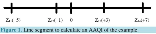
In Figure 1, this study illustrates a simple example to calculate an AAQI. Four measurements Z11, Z12, Z13 and
Z14 are calculated from the first principal component representing the levels of multiple air pollutants. The
length of the line segment for each measurement is as follows: Z Z11 14 =12; Z Z11 12=4; and Z Z11 13=8.
Therefore, the proportions of the four measurements are 0, 0.333 4 12 ,
8 0.666
12
, and 1, respectively. The AAQIs for Z11, Z12, Z13 and Z14 finally are calculated as 0, 33.3, 66.6, and 100, respectively.
4. Data
An AAQI using PCA and the concept of a line segment was developed in Section 3 for multiple air pollutants. Under the Clean Air Act, the USEPA provides air quality standards for the five common air pollutants to sug-gest air quality guidelines to state policy planners and industrial sectors and protect public health [42]. For this reason, the five air pollutants of CO, NOx, PM, SO2, and VOCs were used for the index. Since principal
com-ponents are not scale-invariant, all variables should be measured in the same units [3]; therefore, all variables measured in tons were utilized by each transport mode in the 53 states in the US These were obtained from the NEI of the USEPA in 2008, and were the latest estimated air pollutants available during the study period [48].
Table 1shows the summary statistics for the data utilized in this study. The five air pollutants measured for each transport mode by state do not show any kind of heterogeneity since the coefficient of variation in each va-riable calculated was less than 10 [45]. For the airline transport mode, Texas emits the largest air pollution for each air pollutant, while District of Columbia shows the least air pollution. On the other hand, Idaho emits the fewest air pollutants for vessel and Louisiana shows the largest air pollution in CO, NOx, PM, and VOCs, but
Texas is the largest SO2 emission state. For rail, Nebraska contributes to the largest air pollution across the
na-tion for the four air pollutants, but Texas emits the largest SO2 emission as in the vessel case. For all five air
pollutants, Rhode Island emits the least air pollution. For truck, California is the number one air pollu-tion-emitting state for CO, NOx, and VOCs, while Texas is for PM and SO2. The least air pollution state for NOx,
PM, and SO2 is Idaho, but that for CO and VOCs is Rhode Island.
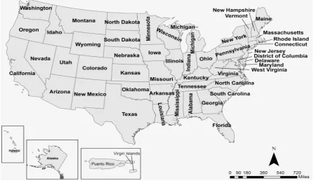
Figure 2 provides a geographic map showing the study area where the five air pollutants were emitted. The NEI provides them by state, but there are no data available for some states for the vessel, rail, and truck transport sectors: Arizona, Colorado, Montana, North Dakota, New Mexico, Nevada, South Dakota, Utah, Virgin Islands, Vermont, and Wyoming in vessel; and Hawaii, Puerto Rico, and Virgin Islands in rail and truck.
5. Empirical Results
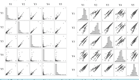
Like most multivariate analyses where the data used follow the multivariate normal (or at least approximately multivariate normal) distribution [46], this study uses a multivariate analysis with PCA. Thus, the developed AAQI tests two statistical assumptions. The first assumption is of multivariate normality. In Figure 3, the scatter plot matrix on the left indicates that the original data do not suggest any normality and even each variable shows
[image:4.595.186.437.643.698.2]Z11(−5) Z12(−1) 0 Z13(+3) Z14(+7)
Figure 1. Line segment to calculate an AAQI of the example.
4Deciding on the number of components followed a recommendation of retaining sufficient components to account for at least 80 percent of
57
Table 1.Summary statistics for the five air pollutants emitted by the four transport modes.
Airline
Pollutant N. of Obs. Mean Std. Dev. Min. Max. CV
CO (tons) 53 8268.350 9963.030 11.979 54029.810 1.205
NOX (tons) 53 2277.850 3401.790 0.266 17043.920 1.493
PM (tons) 53 180.919 211.983 0.272 1145.140 1.172
SO2 (tons) 53 239.642 351.130 0.058 1866.450 1.465
VOCs (tons) 53 625.677 1018.070 0.465 6144.000 1.627
Vessel
Pollutant N. of Obs. Mean Std. Dev. Min. Max. CV
CO (tons) 42 2065.370 4053.190 0.005 23719.810 1.962
NOX (tons) 42 12771.610 23159.440 0.027 132292.350 1.813
PM (tons) 42 645.534 1074.950 0.001 5677.870 1.665
SO2 (tons) 42 3403.410 5582.650 0.002 23870.760 1.640
VOCs (tons) 42 342.995 564.392 0.001 3110.910 1.645
Rail
Pollutant N. of Obs. Mean Std. Dev. Min. Max. CV
CO (tons) 50 2398.720 2082.860 8.592 10858.510 0.868
NOX (tons) 50 16913.600 14342.040 87.267 74404.650 0.848
PM (tons) 50 551.335 476.072 2.148 2484.400 0.863
SO2 (tons) 50 215.729 273.284 0.607 1736.870 1.267
VOCs (tons) 50 883.754 763.524 3.222 3760.480 0.864
Truck
Pollutant N. of Obs. Mean Std. Dev. Min. Max. CV
CO (tons) 50 18677.270 20442.930 918.432 99166.890 1.095
NOX (tons) 50 63501.130 69821.420 2577.990 363276.210 1.100
PM (tons) 50 3524.960 3706.050 159.779 18699.870 1.051
SO2 (tons) 50 92.377 92.783 3.666 467.146 1.004
VOCs (tons) 50 4214.540 4634.510 225.378 24122.660 1.100
Note: All air pollutants data come from the NEI in the USEPA [48].
[image:5.595.90.538.449.707.2]58
a positive skew. On the other hand, after the transformation of the original data5, the right side in Figure 3 shows the approximate normal distribution for each variable. The Q-Q plot for each variable does not show any distinct nonlinear relationship, not indicating a departure from the multivariate normality distribution [40].
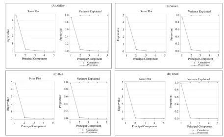
The second assumption is that this study can only use one principal component to sufficiently represent the five air pollutants y y y y y1, 2, 3, 4, 5. To check this, the scree plots and proportion of variance explained by each principal component were tested (see Figure 4). The scree plots in all the transport modes reveal an evident nat-ural break between the first and second principal components. Further, the proportion of the first principal com-ponent calculated6 shows more than 90 percent in each transport, which is much higher than a recommendation of retaining enough components to account for 80 percent of the total variance [40]. Being able to use only a first principal component to explain most of the total variance provides a significantly practical and convenient tool to interpret multiple air pollutants. For example, in the original data in 2008 by airline transport, two states, Iowa and Idaho, emitted the five air pollutants of CO, NOx, PM, SO2, and VOCs as follows: 2679, 272, 59, 37,
and 119 (tons) and 3975, 255, 91, 35, and 147 (tons), respectively. In terms of individual air pollutants, Idaho emitted more (less) air pollution in CO, PM, and VOCs (NOx and SO2) than Iowa, but practitioners, state policy
planners, and the public might want to know the overall air quality level from this kind of conservative situation. The first principal component calculated from the normalized eigenvectors of the sample covariance matrix was used to address this problem.
By using PCA and a little bit of algebra about a line segment with the transformed data, the first principal com-ponent and the AAQI by state in the airline, vessel, rail, and truck transport sectors were calculated, as shown in Table 2and Table 3. In addition, to compare the relative levels of air quality by state from the indices, the state GDP in each transport mode was added in these tables. Each state is ranked relative to all other observed values of states in the first principal component, from smallest to largest in order of magnitude. The rank of each state is denoted by its AAQI. The index increases from 0 to 100, and this indicates more air pollution when it ap-proaches a higher index value. The index of a state showing 100 means the largest air pollution-emitting state of all. On the other hand, a state index indicating 0 implies that the state is the least air pollution-emitting state.
Y1
Y2
Y3
Y4
Y5 Y1
Y2
Y3
Y4
Y5
Y1 Y2 Y3 Y4 Y5 Y1 Y2 Y3 Y4 Y5
[image:6.595.90.534.406.661.2](A) Scatter plot matrix before the transformation (B) Scatter plot matrix after the transformation
Figure 3.Tests for departures from multivariate normality in the data set before and after the transformation.
5In an attempt to make the individual variables distributed more closely to a normal distribution and them distributed more closely to a
mul-tivariate normal distribution, the following variables were used in this study: * 2 1 ln 1
y = y ; * 2
2 ln 2
y = y ; * 2 3 ln 3
y = y ; * 2 4 ln 4
y = y ; and
* 2 5 ln 5
y = y .
59 4 Scree Plot 3 2 1 0
1 2 3 4 5 Principal Component E ige nva lue 4 Scree Plot 3 2 1 0
1 2 3 4 5 Principal Component E ige nva lue 5 4 Scree Plot 3 2 1 0
1 2 3 4 5 Principal Component E ige nva lue 5 4 Scree Plot 3 2 1 0
1 2 3 4 5 Principal Component E ige nva lue 5
1 2 3 4 5 Principal Component
1 2 3 4 5 Principal Component
1 2 3 4 5 Principal Component 1 2 3 4 5
Principal Component 0.0 0.2 0.4 0.6 0.8 1.0 P ropor ti on Variance Explained 0.0 0.2 0.4 0.6 0.8 1.0 P ropor ti on 0.0 0.2 0.4 0.6 0.8 1.0 P ropor ti on 0.0 0.2 0.4 0.6 0.8 1.0 P ropor ti on
Variance Explained Variance Explained Variance Explained
(A) Airline (B) Vessel
(C) Rail (D) Truck
Cumulative Proportion
Cumulative
Proportion Cumulative Proportion
[image:7.595.80.538.80.360.2]Cumulative Proportion
Figure 4.The eigenvalues and proportion of variance explained by the first k principal components by each transport mode (k = 1, 2, 3, 4, 5).
The AAQIs in Table 2and Table 3 are on the ordinal scale; in other words, it is only possible to distinguish each state on the basis of the relative amounts of multiple air pollutants. For instance, in vessel transport in Table 2, the index of Iowa shows 34.01, while that of Kentucky is 70.55. This does not tell us whether the air pollution by vessel in Kentucky is twice more polluted than that in Iowa, but rather it is interpretable in the way that Kentucky shows worse air pollution in terms of considering multiple air pollutants than Iowa. In fact, in 2008 Iowa emitted 151, 786, 27, 46, and 17 (tons) of CO, NOx, PM, SO2, and VOCs, respectively, whereas
Kentucky emitted a considerable amount of air pollutants: 1847, 11370, 441, 594, and 300 (tons).
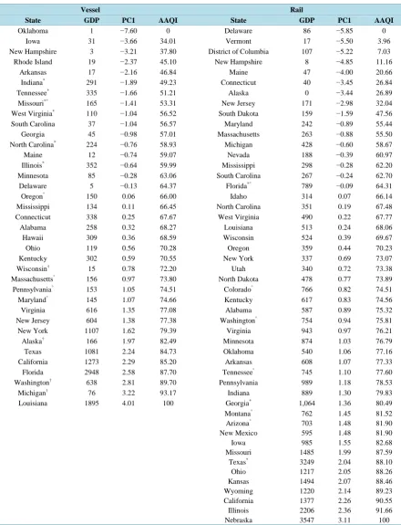
In Table 2, the vessel and rail transport sectors are first analyzed. In vessel transport, Oklahoma is the least air pollution-emitting state, but Louisiana shows the largest air pollution. Indiana, Illinois, Missouri, North Car-olina, West Virginia, and Tennessee account for a relatively low AAQI compared with their high GDP levels, whereas Alaska, Michigan, Wisconsin, and Washington hold high ranks in the AAQI compared with their low GDP levels. For rail transport, Delaware takes the lowest rank in the index and Nebraska accounts for the high-est rank. Florida, Georgia, and Texas show relatively low air pollution against their high GDP level. Massachu-setts, Maryland, Missouri, Oregon, and Pennsylvania in vessel transport, consisting of a similar GDP scale, are differently ranked in the AQI, and this happens to rail transport with Arizona, Colorado, Florida, Montana, Tennessee, and Washington.
60
Table 2. The first principal component and AAQI by state in the vessel and rail transport sectors.
Vessel Rail
State GDP PC1 AAQI State GDP PC1 AAQI
Oklahoma 1 −7.60 0 Delaware 86 −5.85 0
Iowa 31 −3.66 34.01 Vermont 17 −5.50 3.96
New Hampshire 3 −3.21 37.80 District of Columbia 107 −5.22 7.03
Rhode Island 19 −2.37 45.10 New Hampshire 8 −4.85 11.16
Arkansas 17 −2.16 46.84 Maine 47 −4.00 20.66
Indiana* 291 −1.89 49.23 Connecticut 40 −3.45 26.84
Tennessee* 335 −1.66 51.21 Alaska 0 −3.44 26.89
Missouri*° 165 −1.41 53.31 New Jersey 171 −2.98 32.04
West Virginia* 110 −1.04 56.52 South Dakota 159 −1.59 47.56
South Carolina 37 −1.04 56.57 Maryland 242 −0.89 55.44
Georgia 45 −0.98 57.01 Massachusetts 263 −0.88 55.50
North Carolina* 224 −0.76 58.93 Michigan 428 −0.60 58.67
Maine 12 −0.74 59.07 Nevada 188 −0.39 60.97
Illinois* 352 −0.64 59.99 Mississippi 298 −0.28 62.20
Minnesota 85 −0.28 63.06 South Carolina 267 −0.24 62.70
Delaware 5 −0.13 64.37 Florida*° 789 −0.09 64.31
Oregon° 150 0.06 66.00 Idaho 314 0.07 66.14
Mississippi 134 0.11 66.45 North Carolina 351 0.19 67.48
Connecticut 338 0.25 67.67 West Virginia 490 0.22 67.77
Alabama 258 0.32 68.27 Louisiana 513 0.24 68.06
Hawaii 309 0.36 68.59 Wisconsin 524 0.39 69.67
Ohio 119 0.56 70.28 Oregon 359 0.44 70.23
Kentucky 302 0.59 70.55 New York 337 0.69 73.07
Wisconsin† 15 0.78 72.20 Utah 340 0.72 73.38
Massachusetts° 156 0.97 73.80 North Dakota 478 0.77 73.89
Pennsylvania° 153 1.05 74.51 Colorado° 766 0.82 74.51
Maryland° 145 1.07 74.66 Kentucky 617 0.83 74.56
Virginia 616 1.35 77.08 Alabama 587 0.89 75.32
New Jersey 604 1.38 77.38 Washington° 754 0.94 75.81
New York 1107 1.62 79.39 Virginia 943 0.97 76.21
Alaska† 166 1.97 82.49 Minnesota 874 1.03 76.79
Texas 1081 2.24 84.73 Oklahoma 540 1.06 77.16
California 1273 2.29 85.20 Arkansas 608 1.07 77.33
Florida 2948 2.58 87.70 Tennessee° 745 1.10 77.60
Washington† 638 2.81 89.70 Pennsylvania 989 1.18 78.53
Michigan† 76 3.22 93.17 Indiana 889 1.30 79.83
Louisiana 1895 4.01 100 Georgia* 1,064 1.36 80.49
Montana° 762 1.45 81.52
Arizona° 703 1.48 81.90
New Mexico 595 1.48 81.90
Iowa 985 1.55 82.68
Missouri 1485 1.99 87.59
Texas* 3249 2.04 88.10
Ohio 1217 2.05 88.26
Kansas 1494 2.07 88.46
Wyoming 1220 2.14 89.23
California 1377 2.26 90.55
Illinois 2206 2.36 91.66
Nebraska 3547 3.11 100
61
Table 3.The first principal component and AAQI by state in the airline and truck transport sectors.
Airline Truck
State GDP PC1 AAQI State GDP PC1 AAQI
Delaware 18 −5.05 0 Idaho 734 −5.24 0
Virgin Islands N/A −4.48 6.00 Rhode Island 202 −5.24 0.05
Vermont 24 −3.96 11.31 District of Columbia 18 −4.45 8.63
Wyoming 46 −3.47 16.42 Vermont 221 −4.28 10.46
Rhode Island 79 −3.44 16.68 Delaware 232 −3.87 14.94
West Virginia 16 −2.96 21.67 North Dakota* 560 −2.51 29.72
North Dakota 15 −2.51 26.38 Nevada* 683 −2.34 31.62
South Dakota 19 −2.36 27.86 South Dakota* 506 −2.12 33.96
New Hampshire 86 −2.23 29.27 Alaska 285 −2.07 34.51
Maine 43 −2.04 31.19 New Hampshire 289 −1.92 36.13
Montana 59 −1.64 35.38 Wyoming 456 −1.82 37.30
Iowa 58 −1.62 35.58 Montana 441 −1.60 39.71
Connecticut* 270 −1.57 36.09 Maine 490 −1.56 40.11
Nebraska 75 −1.55 36.33 Connecticut 660 −1.50 40.78
Kansas 55 −1.22 39.69 West Virginia 697 −1.10 45.07
Idaho 80 −1.18 40.13 Nebraska* 1,957 −0.41 52.65
Puerto Rico N/A −1.17 40.23 Utah 1,551 −0.28 54.01
New Mexico 163 −0.95 42.56 Kansas 1,508 −0.18 55.17
Mississippi† 38 −0.94 42.57 New Mexico† 700 −0.15 55.41
Arkansas 129 −0.53 46.83 Arkansas* 2,549 −0.06 56.41
South Carolina 110 −0.41 48.14 Iowa* 2,407 −0.03 56.81
Utah 782 −0.28 49.48 Oregon 1,616 0.00 57.03
Oklahoma 723 −0.17 50.65 Mississippi 1,475 0.19 59.12
Oregon 524 0.18 54.20 Colorado 1,634 0.22 59.53
Louisiana° 370 0.21 54.57 Maryland 1400 0.33 60.65
Maryland 622 0.27 55.11 Massachusetts 1462 0.48 62.30
Kentucky 553 0.35 55.99 South Carolina 1584 0.49 62.45
Indiana 493 0.45 57.04 Louisiana 1696 0.57 63.25
Missouri 764 0.60 58.54 Wisconsin° 3767 0.66 64.22
Alabama† 95 0.66 59.24 Alabama 2125 0.75 65.30
Hawaii 1037 0.79 60.52 New Jersey° 3669 0.76 65.35
Nevada 1102 0.81 60.75 Oklahoma 1736 0.94 67.27
Minnesota* 2094 0.96 62.26 Kentucky 1812 1.02 68.14
New Jersey* 2390 1.00 62.70 Virginia 2420 1.18 69.93
Massachusetts† 865 1.00 62.73 Minnesota 2278 1.21 70.28
Virginia 1784 1.44 67.29 Washington° 3767 1.45 72.82
Colorado 1624 1.48 67.66 New York 3388 1.45 72.89
Michigan 1683 1.54 68.32 Arizona 1834 1.59 74.35
Tennessee† 610 1.56 68.54 Missouri° 3646 1.61 74.58
Washington 1489 1.60 68.88 Indiana 4490 1.65 75.10
Pennsylvania 1355 1.61 69.05 Pennsylvania 5493 1.72 75.85
Ohio 1494 1.62 69.19 Tennessee 4702 1.83 77.06
Alaska† 593 1.63 69.23 North Carolina†° 3640 1.85 77.20
Arizona 1888 2.04 73.50 Ohio 5990 2.22 81.22
North Carolina 1309 2.08 73.89 Michigan† 3453 2.38 83.04
Illinois 4510 2.31 76.32 Illinois 6435 2.43 83.51
Wisconsin†° 403 2.35 76.74 Georgia† 3979 2.79 87.42
New York 4223 2.47 77.90 Florida† 4003 3.10 90.83
Georgia 4966 2.69 80.20 Texas 10,926 3.94 99.98
Florida 4120 3.43 87.90 California 11,948 3.94 100
California 6555 4.01 93.86
Texas 7474 4.60 100
62
Louisiana and Wisconsin, showing a similar GDP scale, are differently ranked in the AAQI, which also arises in rail transport with Missouri, New Jersey, North Carolina Washington, and Wisconsin.
6. Conclusions
Transportation is an essential part of the socioeconomic development of a nation, but it has been needed to ac-company the undesirable output called air pollution even though advances in technology for modern transport have contributed to reducing air pollution emissions in comparison with past transport modes. On the other hand, the continuous increase in a clean air environment for public health and sustainable growth between current and future generations has had a positive effect on the transportation sector, corresponding to the growing tide of preserving and improving air quality over the past decades.
An easily understandable tool to measure the level of air pollution in the transportation sector by considering multiple air pollutants might raise awareness about clean air to the public, practitioners, state policy planners, and the government. In this study, an AAQI was developed to help prepare decision makers, which could rank a state according to different levels of multiple air pollutants. In the US empirical case, some states were shown as less polluted or more polluted in terms of the index, although their GDP levels for a transport mode were similar to each other. The authors would carefully guess that a possible hypothesis of these differences might be attri-buted to the degree of the use of eco-friendly transport, strictness of air quality standards, and differences in gasoline prices in their boundaries.
This study, however, has a limitation based on the use of the index developed. The index is only available for one sample, not multiple samples together, since each sample has its own different normalized eigenvectors of the sample covariance matrix according to PCA. Thus, the index value of the same state in different two samples by transport mode, e.g., in 2005 and 2008 if 2005 data were available cannot be theoretically compared with each other. However, one possible advantage of the AAQI developed here is that it can be applied to other nu-merous index development projects, not limited to the transportation sector.
Acknowledgements
This research was supported by Mountain-Plains Consortium, which is sponsored by the US Department of Transportation through its university Transportation Centers Program. The contents are sole responsibility of the authors. The authors would like to thank anonymous reviewers for their constructive comments.
Author Contributions
Jaesung Choi conceived of the research and wrote the paper. Ju Dong Park and Yong Shin Park analyzed the data and performed the multivariate analysis. All authors discussed and commented the results and implications.
Conflicts of Interests
The authors declare no conflict of interest.
References
[1] Kampa, M. and Castanas, E.(2008) Human Health Effects of Air Pollution. Environmental Pollution, 151, 362-367. http://dx.doi.org/10.1016/j.envpol.2007.06.012
[2] Chang, T. and Gross, T. (2014) Particulate Pollution and the Productivity of Pear Packers. http://www.nber.org/papers/w19944.pdf
[3] Zivin, J.S.G. and Neidell, M.J. (2014) The Impact of Pollution on Worker Productivity. http://www.nber.org/papers/w17004.pdf
[4] Greenstone, M. and Looney, A. (2011) We Are What We Breathe: The Impacts of Air Pollution on Employment and Productivity. http://www.brookings.edu/blogs/jobs/posts/2011/05/06-jobs-greenstone-looney
[5] Wyon, D. (2014) The Effects of Indoor Air Quality on Performance and Productivity. http://www.ncbi.nlm.nih.gov/pubmed/15330777
63
[7] Wargocki, P., Wyon, D.P. and Fanger, P.O.(2000) Productivity Is Affected by the Air Quality in Offices. Proceedings of Healthy Buildings, 1, 635-640.
[8] Peck, W. and Harmelink, M. (2014) Transportation Air Pollution. http://trid.trb.org/view.aspx?id=114537
[9] Gorham, R. (2014) Air Pollution from Ground Transportation. http://www.un.org/esa/gite/csd/gorham.pdf
[10] Thom, G.C. and Ott, W.R. (1975) Air Pollution Indices: A Compendium and Assessment of Indices Used in the U.S. and Canada. Ann Arbor Science Publishers, Ann Arbor.
[11] The Federal Interagency Task Force (1976) A Recommended Air Pollution Index. United States Government Printing Office, Washington DC.
[12] Hämekoski, K. (1998) The Use of a Simple Air Quality Index in the Helsinki Area, Finland. Environmental Manage-ment, 22, 517-520. http://dx.doi.org/10.1007/s002679900124
[13] The United States Environmental Protection Agency. Air Quality Index Reporting: Final Rule. http://www.epa.gov/ttn/oarpg/t1/fr_notices/airqual.pdf
[14] Trozzi, C., Vaccaro, R. and Crocetti, S. (1999) Air Quality Index and Its Use in Italy’s Management Plans. Science of the Total Environment, 235, 387-389. http://dx.doi.org/10.1016/S0048-9697(99)00242-9
[15] Sharma, M., Maheshwari, M., Sengupta, B. and Shukla, B. (2003) Design of a Website for Dissemination of Air Qual-ity Index in India. Environmental Modelling & Software, 18, 405-411.
http://dx.doi.org/10.1016/S1364-8152(03)00003-3
[16] Sharma, M., Pandey, R., Maheshwari, M., Sengupta, B., Shukla, B., Gupta, N. and Johri, S. ( 2003) Interpretation of Air Quality Data Using an Air Quality Index for the City of Kanpur, India. Journal of Environmental Engineering and Science, 2, 435-462.
[17] Murena, F. (2004) Measuring Air Quality over Large Urban Areas: Development and Application of an Air Pollution Index at the Urban Area of Naples. Atmospheric Environment, 38, 6195-6202.
http://dx.doi.org/10.1016/j.atmosenv.2004.07.023
[18] Nagendra, S.S., Venugopal, K. and Jones, S.L. (2007) Assessment of Air Quality near Traffic Intersections in Banga-lore City Using Air Quality Indices. Transportation Research Part D: Transport and Environment, 12, 167-176. http://dx.doi.org/10.1016/j.trd.2007.01.005
[19] Wen, X.-J., Balluz, L. and Mokdad, A. (2009) Association between Media Alerts of Air Quality Index and Change of Outdoor Activity among Adult Asthma in Six States, BRFSS, 2005. Journal of Community Health, 34, 40-46. http://dx.doi.org/10.1007/s10900-008-9126-4
[20] Eder, B., Kang, D.W., Trivikrama, R.S., Rohit, M., Shaocai, Y., Tanya, O., Ken, S., Richard, W., Scott, J., Paula, D., Jeff, M. and George, B. (2010) Using National Air Quality Forecast Guidance to Develop Local Air Quality Index Forecasts. Bulletin of the American Meteorological Society, 91, 313-326.
[21] Swamee, P.K. and Tyagi, A. (1999) Formation of an Air Pollution Index. Journal of the Air & Waste Management As-sociation, 49, 88-91. http://dx.doi.org/10.1080/10473289.1999.10463776
[22] Cheng, W.-L., Kuo, Y.-C., Lin, P.-L., Chang, K.-H., Chen, Y.-S., Lin, T.-M. and Huang, R. (2004) Revised Air Quali-ty Index Derived from an Entropy Function. Atmospheric Environment, 38, 383-391.
http://dx.doi.org/10.1016/j.atmosenv.2003.10.006
[23] Cheng, W.-L., Chen, Y.-S., Zhang, J., Lyons, T., Pai, J.-L. and Chang, S.-H. (2007) Comparison of the Revised Air Quality Index with the PSI and AQI Indices. Science of the Total Environment, 382, 191-198.
http://dx.doi.org/10.1016/j.scitotenv.2007.04.036
[24] Kyrkilis, G., Chaloulakou, A. and Kassomenos, P.A. (2007) Development of an Aggregate Air Quality Index for an Urban Mediterranean Agglomeration: Relation to Potential Health Effects. Environment International, 33, 670-676. http://dx.doi.org/10.1016/j.envint.2007.01.010
[25] Bishoi, B., Prakash, A. and Jain, V. (2009) A Comparative Study of Air Quality Index Based on Factor Analysis and US-EPA Methods for an Urban Environment. Aerosol and Air Quality Research, 9, 1-17.
[26] Longhurst, J. (2005) 1 to 100: Creating an Air Quality Index in Pittsburgh. Environmental Monitoring and Assessment,
106, 27-42.
[27] Stieb, D.M., Doiron, M.S., Blagden, P. and Burnett, R.T. (2005) Estimating the Public Health Burden Attributable to Air Pollution: An Illustration Using the Development of an Alternative Air Quality Index. Journal of Toxicology and Environmental Health, Part A: Current Issues, 68, 1275-1288. http://dx.doi.org/10.1080/15287390590936120
[28] Stieb, D.M., Burnett, R.T., Marc, S.-D., Brion, O., Shin, H.H. and Economou, V. (2008) A New Multipollutant, No-Threshold Air Quality Health Index Based on Short-Term Associations Observed in Daily Time-Series Analyses.
64
[29] Mohan, M. and Kandya, A. (2007) An Analysis of the Annual and Seasonal Trends of Air Quality Index of Delhi. En-vironmental Monitoring and Assessment, 131, 267-277. http://dx.doi.org/10.1007/s10661-006-9474-4
[30] Mayera, H., Holsta, J., Schindlera, D. and Ahrensb, D. (2008) Evolution of the Air Pollution in SW Germany Eva-luated by the Long-Term Air Quality Index LAQx. Atmospheric Environment, 42, 5071-5078.
http://dx.doi.org/10.1016/j.atmosenv.2008.02.020
[31] Sowlat, M.H., Gharibi, H., Yunesian, M., Mahmoudi, M. and Lotfi, S. (2011) A Novel, Fuzzy-Based Air Quality Index (FAQI) for Air Quality Assessment. Atmospheric Environment, 45, 2050-2059.
http://dx.doi.org/10.1016/j.atmosenv.2011.01.060
[32] Vyas, S. and Kumaranayake, L. (2006) Constructing Socio-Economic Status Indices: How to Use Principal Compo-nents Analysis. Health Policy Plan, 21, 459-468. http://dx.doi.org/10.1093/heapol/czl029
[33] Soler-Rovira, J. and Soler-Rovira, P. (2008) Assessment of Aggregated Indicators of Sustainability Using PCA: The Case of Apple Trade in Spain. Proceedings of the 6th International Conference on LCA in the Agri-Food Sector, Zu-rich, 12-14 November 2008, 133-143.
[34] Ali Hatem, M.M. (2009) Development of Arab Water Sustainability Index Using Principal Component Analysis. Pro-ceedings of the 13th International Water Technology Conference, Hurghada, 1563-1578.
[35] Li, T., Zhang, H., Yuan, C. and Liu, Z. (2012) A PCA-Based Method for Construction of Composite Sustainability In- dicators. The International Journal of Life Cycle Assessment, 17, 593-603.
http://dx.doi.org/10.1007/s11367-012-0394-y
[36] Hosseini, H.M. and Kaneko, S. (2011) Dynamic Sustainability Assessment of Countries at the Macro Level: A Prin-cipal Component Analysis. Ecological Indicators, 11, 811-823. http://dx.doi.org/10.1016/j.ecolind.2010.10.007
[37] Park, Y.S., Egilmez, G. and Kucukvar, M. (2015) A Novel Life Cycle-Based Principal Component Analysis Frame-work for Eco-Efficiency Analysis: Case of the U.S. Manufacturing and Transportation Nexus. Journal of Cleaner Production, in Press.
[38] Tripping, M.E. and Bishop, C.M. (2002) Probabilistic Principal Component Analysis. Journal of the Royal Statistical Society: Series B (Statistical Methodology), 61, 611-622. http://dx.doi.org/10.1111/1467-9868.00196
[39] Nagendra, S.S. and Khare, M. (2003) Principal Component Analysis of Urban Traffic Characteristics and Meteorolog-ical Data. Transportation Research Part D: Transport and Environment, 8, 285-297.
http://dx.doi.org/10.1016/S1361-9209(03)00006-3
[40] Rencher, A.C. and Christensen, W.F. (2012) Methods of Multivariate Analysis. 3rd Edition, John Wiley & Sons, Inc., Hoboken. http://dx.doi.org/10.1002/9781118391686
[41] Han, B., Bai, Z., Ji, H., Guo, G., Wang, F., Shi, G. and Li, X. (2009) Chemical Characterizations of PM10Fraction of Paved Road Dust in Anshan, China. Transportation Research Part D: Transport and Environment, 14, 599-603. http://dx.doi.org/10.1016/j.trd.2009.07.010
[42] The United States Environmental Protection Agency (2014) Air Quality Trends. http://www.epa.gov/airtrends/aqtrends.html
[43] Choi, J., Roberts, D.C. and Lee, E. (2014) Forecast of CO2 Emissions from the U.S. Transportation Sector: Estimation from a Double Exponential Smoothing Model. Journal of the Transportation Research Forum, 53, 63-82.
[44] The United States Environmental Protection Agency (2014) Air Pollution and the Clean Air Act. http://www.epa.gov/air/caa/
[45] Mendenhall, W. and Sincich, T. (2011) A Second Course in Statistics: Regression Analysis. 7th Edition, Prentice Hall, Upper Saddle River, 797.
[46] Ramzan, S., Zahid, F.M. and Ramzan, S. (2013) Evaluating Multivariate Normality: A Graphical Approach. Middle- East Journal of Scientific Research, 13, 254-263.
[47] The United States Bureau of Economic Analysis (2014) Industry Data. http://www.bea.gov/iTable/index_industry_gdpIndy.cfm
65 Appendix A.Summary of the literature on changes to air quality indices.
Author(s) Year Study area Pollutants measured Methodology Objective(s)
Thom and Ott 1975 US and Canada
CO, NOX, Oxidants,
PM, and SO2 Standardized AQI Developing a uniform AQI Federal Interagency
Task Force 1976 US
CO, NOX, O3, SO2,
and TSP7 PSI
Developing an AQI to report daily air quality by state
Hämekoski 1998 Finland CO, NOX, O3, PM,
and SO2 PSI Applying a PSI in the Helsinki area, Finland Swamee and
Tyagi 1999 India
CO, Haze, NOX, O3, SO2, and TSP
Ambiguity- and eclipsicity-free function
Developing an overall AQI from the aggregation of air pollution sub-indices
Trozzi et al. 1999 Italy CO, NOX, O3, PM,
and SO2 AQI
Applying an AQI developed by the USEPA for Italy
USEPA 1999 US CO, NOX, O3, PM,
and SO2 AQI
Revisions from the PSI to provide additional air quality information
Sharma et al. 2003A India CO, NOX, O3, PM,
and SO2, and SPM8 AQI
Describing the design of a website for the dissemination of AQIs
Sharma et al. 2003B India CO, NOX, O3, PM,
and SO2, and SPM AQI
Applying an AQI developed by the USEPA for the City of Kanpur, India
Cheng et al. 2004 Taiwan CO, NOX, O3, PM, and SO2 Revised AQI (RAQI) Developing an RAQI as combining a PSI with an entropy function
Murena 2004 Italy CO, NOX, O3, PM, and SO2 AQI Implementing an AQI in the urban area of Naples to measure the level of air pollution
Longhurst 2005 US SO2 and particulates Simple formula9 Presenting the case study of an AQI in Pittsburgh, Pennsylvania
Stieb et al. 2005 Canada CO, NOX, O3, PM, and SO2
Time series regression on five air pollutants on mortality
Developing an alternative AQI to illustrate the public health burden attributable to air pollution
Cheng et al. 2007 Taiwan CO, NOX, O3, PM,
and SO2 RAQI
Comparisons between an RAQI and a PSI or AQI for evaluating the feasibility and effectiveness of several air pollution conditions
Kyrkilis et al. 2007 Greece CO, NOX, O3, PM,
and SO2 AAQI
Calculating potential health effects considering five criteria pollutants Mohan and
Kandya 2007 India
CO, NOX, O3, PM,
and SO2 AQI
Measuring the annual and seasonal variations of AQI from 1996 to 2004
Nagendra et al. 2007 India
Ammonia, CO, lead, NOX, O3, SO2, SPM, and RPM10
AQI
Assessing the level of ambient air quality at traffic intersections in Bangalore, India using an AQI developed by the USEPA
Mayer et al. 2008 Germany Benzene, NOX, PM,
and SO2 Long-term AQI (LAQI)
Analyzing the effect of the integral long-term air pollution for 1985-2005
Stieb et al. 2008 Canada CO, NOX, O3, PM, and SO2
Air quality health index (AQHI) using time series regression on five air pollutants on mortality
Developing an AQHI and applying it in multiple Canadian cities
Bishoi and Jain 2009 India CO, NOX, O3, PM, and SO2
New AQI (NAQI) with factor analysis
Comparing an NAQI to an AQI developed by the USEPA
Wen et al. 2009 US CO, NOX, O3, PM,
and SO2 AQI
Studying the relationship between media alerts of AQI and level of outdoor activity
Eder et al. 2010 US CO, NOX, O3, PM,
and SO2 AQI
Developing local AQI forecasts using an AQI developed by the USEPA
Sowlat et al. 2011 Iran
CO, NOX, O3, PM, SO2, benzene, toluene, ethyl-benzene, xylene, and 1, 3-butadiene
Fuzzy-based AQI (FAQI)
Developing a FAQI based on the computational method of artificial intelligence and assessing the performance of the index as a case study of Iran
7TSP stands for total suspended particulates. 8SPM stands for suspended particulate matter.
9
Simple formula is as follows: 50 SO 0.14
(
( 2 ) (+ COH 1.73))
, where SO2 represents its measurement and COH means the coefficient of haze; thedenominators in the formula are based on National Ambient Air Quality Standards [26]. 10