http://dx.doi.org/10.4236/wjm.2014.412035
Sheet Bending Deformation in Production
of Thin-Walled Pipes
Tatjana V. Brovman
Tver State Technical University, Tver, Russia Email: [email protected]
Received 23 September 2014; revised 17 October 2014; accepted 11 November 2014
Copyright © 2014 by author and Scientific Research Publishing Inc.
This work is licensed under the Creative Commons Attribution International License (CC BY). http://creativecommons.org/licenses/by/4.0/
Abstract
Nowadays, thin-walled super-diameter pipes are produced by the method of plastic bending of sheets. After a sheet is bent into a pipe and its ends are welded, a pipe billet is subjected to expansion deformation. The technology of forming end areas of a sheet is developed and formu- laes forming forces equations are deduced. Experimental investigations of deformation are under- taken.
Keywords
Plastic Deformation, Bending of Billets, Calculation of Forming Forces, Quality of Pipes
1. Introduction
Nowadays thin-walled pipes are made of metal sheets by the method of plastic bending in terms of the required diameter with the following welding of edges by a longitudinal seam [1] [2].
Sometimes two half-cylinder billets are bent with the following welding by two longitudinal seams.
Elastoplastic bending is used for production of high-strength steel pipes of super-diameter (1020 - 1420 mm and more), with the length being up to 18 metres and wall thickness to 40 - 55 mm. Bending is produced by the “step-by-step forming” method, with the sheet being moved after every strain cycle.
Since dimensional accuracy of pipes thus produced is low, end areas of sheets are stamped, (pressed by two curved dies) [2]-[4].
The choice of technological modes, however, is hampered by the lack of formulas to calculate the required parameters of bending in view of residual deformations. Besides, there are no experimental data on the intensity of sheet deformation in dies.
sheets.
[image:2.595.175.403.416.683.2]2. Relation of Deflection of Billet to Be Formed and Value of Its Bending Flexure
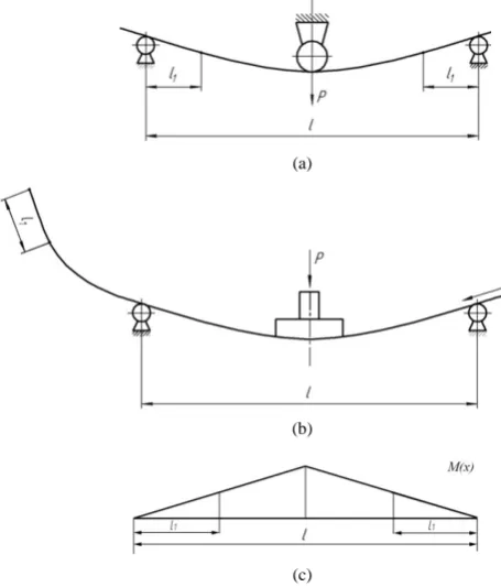
Figure 1shows a diagram of bending the billet at the length l produced by a pressure roller (Figure 1(a)) or a punch (Figure 1(b)).When a sheet of width b and thickness h is bent by force P, in most cases one can use the model of an ideal elastoplastic body with constant yield point σT and modulus of elasticity E.
In this case two dimensionless parameters, as per [5], are inserted to the methods of calculation of elastoplas-tic bending
2, 4
Т
T
l Pl
m n
Eh bh
σ σ
= =
where the first one characterizes a ratio between the force (and the maximum bending moment) and the limit plastic moment, while the second—a ratio of elastic and plastic properties of metal.
Figure 1(с) shows a bending moment diagram М(х), where х is a longwise coordinate of a billet. Maximum bending moment 0.25 Рl acts in the middle of the billet length where force P is applied. Maximum deflection in the cross section х = 0.5l is calculated by the standard method [3] [4]. It is equal to
(
)
2
0.024
0.96 1 2 1 4
m m
V
al m m
= − + −
(1)
If, for example, a metal sheet with yield point σ =T 300МН m2, modulus of elasticity
5 2
2 10 МН m
E= × ,
length l = 1 m and thickness h= ×4 10−2m, then value Vm 0.2
al = under the load defined by parameter m = 0.2.
At present value 2
5 2
300 1
3.75 10 2 10 4 10
a= × − = × −
× × × deflection at the midpoint of a billet is equal to
(a)
(b)
(c)
Figure 1. Bending deformation diagrams: (а) Bending by pres-
3 7.5 10 m m
V = × − .
Formula (1) is may be used only in the range of 1 1 6≤ ≤m 4, if
1 6
m= , then Vm =0.167аl (but if 1 6 m< ,
linear dependence Vm m
al = is valid).
In the course of bending the value of maximum curvature is attained if х=0.5l (Figure 1).
2 1
3 1 4 m a K l m = −
(2)
However, after off-loading which occurs under elastic deformation, the residual curvature of a billet is equal to
0
2 1
6 3 1 4 a K m l m = − −
(3)
If а=3.75 10× −2 and m = 0.2
2
2 1
2 3.75 10 1
9.7 10 ,
1 3 0.2
m K m − − − × = × = × 2 2 0
2 3.75 10 1
1.2 0.68 10
1 3 0.2
K m − − × × − = × × =
It is seen that value K0 is much less than Km. With increase of m=0.24, 1 0 1.45
K = m− i.e. the flexure increases 2.1 times (compared to the load when m = 0.2).
If 1 6
m≤ , only elastic deformations take place. So if 1 6
m= , K0 =0 and the residual curvature is equal to
zero (value Km 2a l
= when 1 6
m= ). If bending moment tends to limiting value 1 4
m= , Km → ∞ and
0
K → ∞.
In the conditions of elastoplastic medium without hardening and σ =Т const, plastic deformation billet at
the surface of a stock in the middle of its length, and this area will expand with the increase of load. If 1 4 m= ,
plastic deformation (in the center of a billet) will cover the whole section and this means the loss of billet bear-ing capacity (for the material without hardenbear-ing).
Function graph Vm
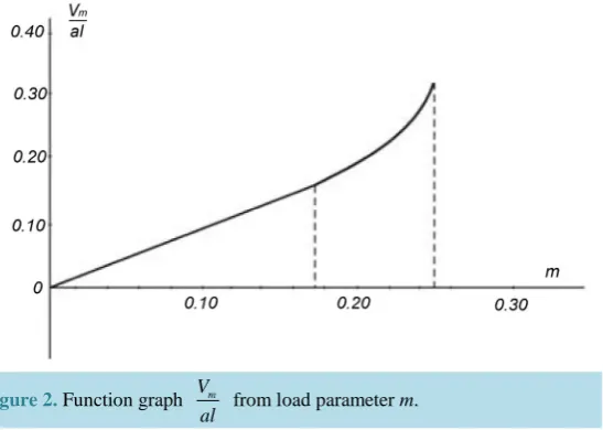
al from load parameter m is given in Figure 2. It is seen that the rate of deflection in- creases when m → 0.25.
However, near the ends of the sheets to be bent there are sections l1 (Figure 1) where plastic deformation is not possible. Their length is:
1 12 l l m =
Since a limiting value of non-dimensional load parameter 1 4
m= , minimum length 1 3 l
l = . This means that
plastic bending deformation under the diagram of Figure 1 can be performed only along the length equal to one-third of the total billet length, i.e. the distance between supports.
According to the bending diagram of Figure 1(a), two-thirds of a billet length remains straight. According to the step-by-step bending diagram of Figure 1(b), a billet is gradually moved then brought to stop in order to be bent and it again keeps approaching as shown by the arrow. Each approach step should not be greater than value
3 l
Figure 2. Function graph Vm
al from load parameter m.
the dimensional accuracy of a molded pipe (or a bent billet).
In this process, in contrast to a single-step bending (Figure 1(a)), the dimensional accuracy of a billet is high-er, but segments of length l1remainstill straight (Figure 1(b)) at the nose and butt ends of a billet.
This will make a billet or a pipe after bending deformation be configured as shown inFigure 3.
It does not make much difference in manufacturing ring billets used in mechanical engineering, for example straps, especially if they are machined anyhow.
However, flat areas in manufacturing pipes greatly reduce their quality. As noted in [3], differences in diame-ter values (their nominal values 1000 - 1500 mm) can reach 8 - 15 mm, and these pipes are often unsuitable for pipelines.
Therefore, many large-diameter pipe manufacturers use the SMS MEER technology as per which end areas of sheets (edges) are bent by a flanging machine. After welding pipe billet is subjected to internal expanding by pressure of 12 wedges. First an arbor with wedges is got into the pipe, and then radial movement of wedges ex-erts pressure on the inner surface of pipe and increases its diameter, thus reducing flexure fluctuations. However, the pressure near А and В (Figure 3) can result in plastic deformation near weld zone С. Microcracks can appear
in the zones under substantial tensile stress near pipe inner surface during expansion. The presence of residual stress is also important. There are some facts (see [3]) that most fractures of X70 steel pipes of 1420 mm diame-ter at gas pipelines occur on areas up to 200 mm from a longitudinal weld. It is clear that the pipes with two lon-gitudinal welds do not have two flat areas, as shown in Figure 3, but four ones and so twice higher possibility of defect development when expanding.
That is why the quality of such pipes compared with single-weld ones is lower. Pipe stress-relief tempering at 250˚C - 300˚C during two hours is sometimes recommended to prevent stress-corrosion [3].
However, tempering reduces residual stress but cannot help in cases of developing microcracks or delamina-tion during pipe diameter expansion. In addidelamina-tion, such tempering leads to high energy consumpdelamina-tion up to 1.8 - 2.0 МJ per a metric ton of pipes. In consideration of large pipe length (up to 10 - 12 m and more) the energy consumption will be two-three times higher due to losses.
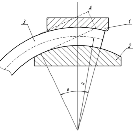
Thus, it is highly desirable for end areas of billets to be compressed between dies as shown in Figure 4. The above mentioned process is used in practice which is, however, difficult because of the lack of experi-mental data on the intensity of stress for deformation in forming sheet stock end areas.
3. Force Determination in Stock End Area Die Forming
The initial position of a stock end area is indicated by a dotted line in Figure 4. Firstly, a moving die contacts line А (Figure 4), then bends the section which envelopes the surface of a counter die. Dies 1 and 2 come closer
and deform stock 3 so that it forms the curvature K 1 R
Figure 3. Diagram of flat sections in pipe forming.
Figure 4. Deformation diagram of sheet end area in compre- ssing between dies.
Provide the parameters determining the intensity of force, with their dimensions given in brackets: R (m), h (m), σТ (N/m2), b (m), l (m), Р (N), where Р is deformation force.
The parameters can be used to make four dimensionless parameters
1 , 2 , 3 , 4 .
T
l h b P
A A A A
R l R σ bl
= = = =
According to π theorem the relation of the indicated parameters must be in the form
(
1, 2, 3, 4)
0F A A A A =
or, if it is solved relative to А4, we can derive А4= f
(
А А А1, 2, 3)
or(
1, 2, 3)
TP=σ blf А А А (4)
[image:5.595.201.431.285.508.2], T
P blf h l
l R
σ
=
(5)
To determine the upper limit of capacity and force values, a kinematically admissible velocity field was used (in polar coordinates)
(
)
(
)
0, , ,
r z
V = Vθ =c r rθ −R V = −cz r−R
where , ,rθ z are coordinates, c is a constant, R is a stock mean radius (its neutral axis). The components of deformation velocity tensor are determined by conventional equations, see [4].
(
)
(
)
0, , ,
r θ c r R z c r R
ε = ε = − ε = − − and form change capacity
0.5 0.5 0.5
0.5 d 0.5 d 0.5 d
3
b R h T
b R h
N z α Hr r
α
σ
θ
+ + +
− − −
=
∫
∫
∫
(6),where the second invariant of deformation velocity tensor is
(
) (
2) (
2)
2 2 2 22
3 r z z r rz r z
H= ε −εθ + εθ−ε + ε −ε +γ +γθ+γθ
,
where γ γ γrz, rθ, θz are the components corresponding to shear strain.
Numerical calculations, according to (6), show the possibility of the approximate description of function N in the form of
2 2 3 3 T
N =
σ
bhω
where 0
α ω
τ
= is the mean angular velocity of bending an end area and τ0 is the time of forming a sheet billet
end area.
Hence we derive the equation
2 4 3 3 Tbh P l σ
= (7),
which matches relation (5) with
2
4
, .
3 3
h l h
f
l R l
=
To verify the given equations experimental investigations were conducted. They measure the forces deforma-tion of billet ends was made on the press with 1 MN force for steel sheets, with yield strength being 260 МN/m2, the width of sheets being b = 0.6 m and thickness – h = 5 × 10‒3 m, 10 × 10‒3 m and 20 × 10‒3 m. In addition pa-rameters l and R in ranges l = 0.2 - 0.9 m and R = 0.2 - 1.1 mwere changed in the tests. The part of experimen-tal data for sheets of 0.6 m width and the three thicknesses is given in Table 1 with l = 0.9 m, l = 0.4 m and l = 0.2 m.
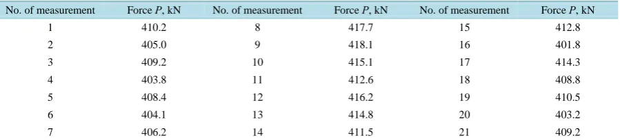
Table 2shows the data on the results of the force measurement with b = 0.6 m, l = 0.4 m and h = 4 × 10‒2 m for the same carbon steel with σT= 260 МN/m2. The average value of the force is: 409.93 kN, the dispersion being 21.3(kN)2.
Thus a standard deviation is 4.62 kN and, following “the rule of three standard deviation”, can be surely as-sumed (with high probability of 0.997) that the intensity of force is in the range of 409.93 ± 3 × 4.62 or 396 - 424 kN. The range of 28 kN or 0.066Pm matches the possible oscillations of formation intensities of force. Dev-iations of (7) type equations up to 20% - 25% are to be taken into consideration in choosing and designing the equipment for forming pipe end areas.
General Equations of (4) and (5) form based on the dimensional theory should be specified with further expe-rimental studies.
If Equation (3) takes the function
2
2
, 0.77
h l h
f
l R l
=
Table 1. Values of force in bending.
l = 0.9 m
Sheet thickness, mm h = 5 mm h = 10 mm h = 20 mm
No. of measurement 1 2 3 1 2 3 1 2 3
Force Р, kN 3.30 3.15 3.08 13.1 12.9 13.4 49.5 52.1 48.7
l = 0.4 m
Sheet thickness, mm h = 5 mm h = 10 mm h = 20 mm
No. of measurement 1 2 3 1 2 3 1 2 3
Force Р, kN 7.08 7.21 7.18 29.8 30.1 29.4 110.1 117.7 108.3
l = 0.2 m
Sheet thickness, mm h = 5 mm h = 10 mm h = 20 mm
No. of measurement 1 2 3 1 2 3 1 2 3
Force Р, kN 14.8 13.9 13.1 59.8 58.3 60.1 235.2 237.4 229.9
[image:7.595.90.540.295.397.2]Stock End Areas, (with b = 0.6 m; σТ = 260 МN/m2; R = 1 m).
Table 2. Values of Force in forming sheet end areas (b = 0.6 m; σТ= 260 МN/m2; l = 0.4 m; h = 4 × 10‒2 m).
No. of measurement Force Р, kN No. of measurement Force Р, kN No. of measurement Force Р, kN
1 410.2 8 417.7 15 412.8
2 405.0 9 418.1 16 401.8
3 409.2 10 415.1 17 414.3
4 403.8 11 412.6 18 408.8
5 408.4 12 416.2 19 410.5
6 404.1 13 414.8 20 403.2
7 406.2 14 411.5 21 409.2
we will derive Equation (7) according to which function f only depends on one dimensionless parameter h l .
But with small values of l
R the parameter also has influence. With 0.4 l
R< the following equation can be used
2 2
5
2 2
, 0.70 10
h l h R
f
l R l l
−
= +
,
For example, with h 0.05
l = ; 5
R
l = ; l = 0.2 m
2 2 3
, 0.70 0.25 10 0.025 10 2 10
h l f l R − − − = × × + × = ×
and force Р=260 0.6 0.2 2 10× × × × −3 =62.4 kN.
With the increase of l
R from 0.2 to 0.4 with the same value of
2 5 10 h l − ×
= the second member decreases
to the magnitude not exceeding 5% of force. Hence, in forming pipes one should not leave too short l 0.3 - 0.4
R
<
flat areas of sections because they are more difficult to be bended in order to get the necessary flexure.
due to discharge in the zone of bending moment decrease so different equations should be used for calculating deflections at these zones.
4. Conclusions
1) The elastoplastic deformation of bending leaves flat areas in billets. It should be deformed to provide the constancy of the curvature along the pipe section. Thus, the formation of sheet end areas is necessary.
2) In bending the billet flat areas to get the necessary flexure (diameter), the choice of step-by-step forming
press forces should be subjected to experimental data results and it is desirable to take parameter l
R not less than 0.4.
References
[1] Rymov, V.А., Polykhin, P.I. and Potapov, I.N. (1983) Improvement of Welded Pipe Production. Metallurgiya, Mos- cow, 307 p.
[2] Barabantsev, G.Ye., Tyulyapin, A.N., Kolobov, A.V. and Yusupov, V.S. (2005) Improvement of Electric-Welded Straight-Line-Seam Pipe Production Technology. Rolled Metal Production, 12, 21-23.
[3] Shinkin, V.N. (2013) Strength of Materials for Metallurgists. Textbook for Higher Schools, DomMISiS Publishing House, Moscow, 655 p.
[4] Hill, R. (1950) Mathematical Theory of Plasticity. Clarendon Press, Oxford, 407 p.