Direct Torque Control of Induction Motor Drive By using Fuzzy Logic Controller and Feedback Linearization Technique

Themed Section: Science and Technology

Direct Torque Control of Induction Motor Drive By using Fuzzy Logic

Controller and Feedback Linearization Technique

Areti. Gopi1_{, J. Nageswara Rao}2_{, G. Satish}3

1 _{PG Scholar, Department of EEE, Nova College of Engineering & Technology, Jupudi, Andhra Pradesh, India}

2_{Assistant Professor, Department of EEE, Nova College of Engineering & Technology, Jupudi, Andhra Pradesh,}

India

3_{HOD, Department of EEE, Nova College of Engineering & Technology, Jupudi, Andhra Pradesh, India}

ABSTRACT

This paper presents a Direct Torque Controlled (DTC) Induction Motor (IM) drive that utilizes feedback linearization and Sliding-Mode Control (SMC). Another feedback linearization approach is proposed which is Fuzzy logic controller (FLC), which outputs a decoupled direct IM display with two state factors: torque and stator flux. This inherent linear model is utilized to actualize a DTC sort controller that preserves all DTC favorable circumstances and takes out its primary disadvantage, the flux and torque swell. Robust, quick, and swell free control is accomplished by utilizing FLC with corresponding control in the region of the sliding mode. Fuzzy logic controller guarantees robustness as in DTC, while the corresponding segment robustness out the torque and flux swell. The torque time reaction is like traditional DTC and the proposed arrangement is adaptable, profoundly tunable because of the P component. The controller design is displayed and its robustness solidness is analyzed in simulations. The FLC controller is contrasted and a direct DTC scheme with and without Feedback linearization. By using FLC controller extensive investigative comes about for dynamic response of a sensorless IM drive approve the proposed solution.

Keywords : Direct Torque Control, Adjustable Speed Drives, Feedback Linearization, Induction Motor Drives, Sliding Mode Control, Fuzzy Logic Controller

I.

Direct Torque Control (DTC) is a robust, quick responding control technique for Induction Machine (IM) drives [1]. Customary DTC utilizes shut circle hysteresis torque also, flux controllers and a changing table to choose the voltage vector connected to the motor. DTC accomplishes quick and robust torque and flux control without utilizing current controllers. DTC operation is related with expansive torque swell which causes ripple, vibrations, and expanded misfortunes, while the switching frequency of the Voltage Source Inverter (VSI) is variable and low. Enhanced DTC arrangements that keep running at

consistent switching frequency and utilize present day control hypothesis have as of late been created to reduce the torque ripple. Novel DTC procedures in light of discrete Space Vector Modulation (SVM) techniques are portrayed in. DTC in light of linear torque and flux controllers (Linear DTC) and SVM was presented in [2]. A few designs utilizing the variable structure control standards have been proposed in [3].

and afterward utilize the opposite change to acquire the desired controller for the first nonlinear system. Since the technique is touchy to displaying errors and disturbances, it has been once in a while connected to IM drives. FBL is utilized as a part of [4]-[5] to linearize the IM display with regard to speed, flux, and current. Two linearization designs in which just a single control amount is changed are discussed about in [5]. All arrangements in [4]-[5] depend on current linearization and control. Utilizations of FBL to control devices and PMSM drives are displayed. An error affectability investigation in demonstrates that the control performance may fall apart because of perturbations, parameter detuning, and estimation errors.

Sliding Mode Control (SMC) is a robust control strategy appropriate for control systems with uncertainties or demonstrating errors [6]. It has been effectively connected to IM drives and gives superb dynamic performance to a wide speed extend operation [3]. The switching conduct can be directed with the VSI operation as appeared in [6]. Fact be told, the customary DTC is a type of SMC which was composed to nearly direct the switching idea of the VSI.

This paper proposes another DTC controller that incorporates Feedback linearization together with fuzzy logic controller (FLC). The principle preferred advantage of FBL over traditional DTC is that the linear control hypothesis results can without much of a extend be connected to acquire a superior performance. We utilize this property to design and after that hypothetically explore the robustness and dependability of the proposed control strategy. Besides, the controller-spectator division rule enables the controller and the spectator to be autonomously designed, if the design display is around linear and estimation errors are small. The FBL load is the affectability of the linearized model to uncertainties

and parameter detuning, which motivates the utilization of FLC.

The nonlinear IM demonstrate considered in this paper is fourth arrange with the state factors: torque, stator flux, rotor flux, described more, another flux subordinate state. The feedback linearized IM show is second order, with just the torque and stator flux magnitude as decoupled state factors. In this way, the new direct display is natural, extremely linear forward, and it generously rearranges the controller design. The flux and torque are controlled by the new DTC conspire and the proposed controllers utilize FLC to keep up robustness sensorless operation of the drive. This approach in light of torque-flux linearization and control is not the same as existing techniques in [4]-[5], which are based on current control. The mix of these systems preserves the quick and robustness reaction of traditional DTC while altogether taking out the torque and flux ripple.

II.

Regular linearization of a nonlinear system depends on a first-arrange estimation of the system dynamic at a chosen working point while dismissing high-arrange flow. This linearization is satisfactory in numerous applications where typical system operation stays in the region of a settled or gradually differing balance, however it is generally wrong. In specific, linearization is proper for IM drives working at consistent rotor speed. Something else, the IM conduct is intrinsically nonlinear and different methodologies must be utilized.

comprehensively, as opposed to in the region of a harmony point. When all is said in done, the linearizing change is very hard to discover, however at times it is anything but difficult to acquire by a basic redefinition of factors [7]. Fortunately the FBL of an IM is achievable by a natural change of the state factors and an info redefinition.

The IM state space show in the stator reference design is

( )

( ) ( )

s r are stator and rotor flux space vectors, Rs and Rr are the stator and rotor resistances, Ls, Lr and Lm are the stator, rotor and magnetizing inductances, 𝑇𝑠 = 𝐿𝑠 /𝑅𝑠, 𝑇𝑟 = 𝐿𝑟 /𝑅𝑟 , 𝜎 = (𝐿𝑠𝐿𝑟 – 𝐿𝑚

2)/𝐿𝑠𝐿𝑟 r is the rotor speed, and 𝑢𝑠 = 𝑢𝑠𝑑 + 𝑗𝑢𝑠𝑞 is the stator voltage vector which acts as Feedback. The model can be linearized by selecting the new states:

𝑀 = 𝜓𝑠𝑞𝜓𝑟𝑑 – 𝜓𝑠𝑑𝜓𝑟𝑞 (3)

𝑅 = 𝜓𝑠𝑑𝜓𝑟𝑑 + 𝜓𝑠𝑞𝜓𝑟𝑞 (4)

𝐹𝑠 = 𝜓𝑠𝑑2 + 𝜓𝑠𝑞2 (5)

𝐹𝑟 = 𝜓𝑟𝑑2 + 𝜓𝑟𝑞 (6)

Where 𝑀 is the scaled torque, Fs and Fr are the squared extents of the stator and rotor flux, individually. The variable 𝑅 relies upon the rotor and stator flux. For linear forwardness, we refer M as the torque and Fs as the flux size. We are essentially intense on controlling the torque 𝑀 and the stator flux flux 𝐹𝑠. In any case, we should likewise safeguard that the remaining state factors, Fr and R, are limited. The IM state conditions with the state factors (3) - (6) are − ( + ) 𝑀 − 𝜔𝑟𝑅 − 𝜓𝑟𝑞𝑢𝑠𝑑 + 𝜓𝑟𝑑𝑢𝑠𝑞 (7) = − 𝐹𝑠 + 𝑅 + 2𝜓𝑠𝑑𝑢𝑠𝑑 + 2𝜓𝑠𝑞𝑢𝑠𝑞 (8)

= − (9)

= − ( + ) 𝑅 + 𝜔𝑟𝑀 + 𝐹𝑠 + 𝐹𝑟 +𝜓𝑟𝑑𝑢𝑠𝑑 + 𝜓𝑟𝑞𝑢𝑠𝑞 (10)

The first three state equations are feedback linearized if the Feedbacks redefined as 𝑤𝑞 = −𝜔𝑟𝑅 − 𝜓𝑟𝑞𝑢𝑠𝑑 + 𝜓𝑟𝑑𝑢𝑠𝑞 (11)

𝑤𝑑 = 𝑅 + 2(𝜓𝑠𝑑𝑢𝑠𝑑 + 𝜓𝑠𝑞𝑢) (12)

Now the linearized system is − ( + ) 𝑀 +wq (13)

= − 𝐹𝑠 +wd (14)

= − (15)

= − ( + ) 𝑅 + 𝐹𝑠 + wd- wq (16)

Solving (11) and (12) gives the control signals usd= ( ) ( ) (17)

usq= ( ) _{( ) (18)}

FBL decouples the state factors of interest; specifically, the torque 𝑀 and the stator flux 𝐹𝑠 and in this manner fundamentally improves the controller design for the IM drive system. In expansion, since the subsequent system is linear, the traditional linear control approaches can be utilized. Since the 𝑀, 𝐹𝑠 and 𝐹𝑟

lower bound, Rl. 𝑅 is likewise upper limited practically speaking on the grounds that the flux extents are restricted because of attractive immersion.

III.

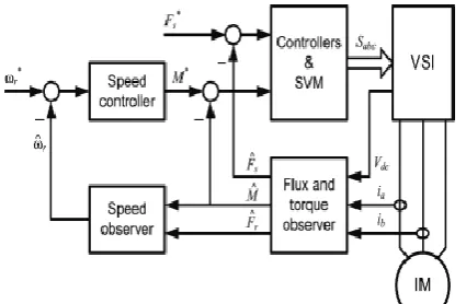
Sliding Mode Control (SMC) is utilized to accomplish a quick and robust operation of an IM drive. Fig. 1 demonstrates the block diagram of the proposed drive. The block Controllers and SVM contains the FBL and the torque and flux controllers portrayed next. The drive utilizes linear forward speed, torque, and flux observer, described more, a PI speed controller. Drive information and a concise representation of the spectators are given in the Appendix.

The control objective is to control the torque and stator flux level in the machine, i.e. to understand a DTC sort controller. To this end, we design controllers for the torque M described more, the stator flux Fs in the linearized demonstrate. Since the state conditions (13) and (14) representing M and Fs individually are decoupled, the design of their controllers to acquire the data sources 𝑤𝑑 and 𝑤𝑞 is very linear forward. These are then substituted in (17) described more, (18) to acquire the physical sources of info 𝑢𝑠𝑑 and 𝑢𝑠𝑞 separately. Be that as it may, errors in the computation of the physical sources of info are unavoidable and must be represented and corrected to give controlling performance.

The errors in the physical control sources of info can be represent to as proportionate errors in the direct state conditions (13) and (14).

Condition (13) can be reworked in the frame

Gm+wq (19)

Where 𝑔𝑀 represents the uncertain dynamics of the FBL torque equation. The term 𝑔𝑀 is not exactly known; from (13) an estimate of the dynamics

Is ̂M= (

)

We assume that the estimation error for 𝑔𝑀 is bounded as

|𝑔 𝑀 − 𝑔𝑀| ≤ 𝐺𝑀 (20)

To design the SMC for the linear system of (19), we define the sliding mode as the torque error

𝑆𝑀 = 𝑀 − 𝑀𝑑 (21)

For this choice of sliding mode, we use the SMC

𝑤𝑞 = −𝑔 𝑀 – 𝑘𝑀 sgn (𝑆𝑀), 𝑘𝑀 > 0 (22)

The term −𝑘𝑀sgn (𝑆𝑀) is known as the corrective control.

We choose the quadratic Lyapunov function candidate 𝑉 = 𝑆𝑀 2 /2. The system converges to the sliding mode if the derivative of a Lyapunov function is negative along all the trajectories of the system. The derivative of V is

𝑆𝑀2 = (𝑔𝑀 − 𝑔 𝑀 − 𝑘𝑀sgn (𝑆𝑀)) = (𝑔𝑀 − 𝑔 𝑀)

−𝑘𝑀|𝑆𝑀| (23)

For robust convergence to the sliding mode the derivative must remain negative in the presence of uncertainties. We choose the corrective control gain

𝑘𝑀 as in eq. (24).

Fig. 1 Block diagram of the sensorless DTC IM drive with feedback linearization.

Fig. 2 Torque and flux SMC with feedback linearization for IM control.

This gives the sliding condition, eq. (25)

𝑆𝑀

2 _{≤ −𝜂𝑀|𝑆𝑀| (25)}

Where 𝜂𝑀 is a positive constant. The gain 𝑘𝑀 of (24) includes the term 𝐺𝑀 to ensure robust stability and the term 𝜂𝑀 to control the speed of convergence to the sliding controller. A bigger 𝜂𝑀 makes the system trajectory to reach the sliding mode in a shorter time but can result in higher chattering. Similar results can be obtained by using an integral sliding mode

𝑆𝑀 = ( + 𝜆𝑀) ∫ ( ) (26)

Where 𝜆𝑀 is a positive constant design parameter. This parameter determines how fast the error goes to zero once the State is on the mode. The SMC effort can be chosen as

𝑤𝑞 = −𝑔 𝑀 − (𝑀 −) − 𝑘𝑀sgn (𝑆𝑀), 𝑘𝑀 >0 ( (27)

and the sliding condition holds for 𝑘𝑀 = 𝐺𝑀 + 𝜂𝑀. To avoid chattering we define a boundary layer around the sliding mode, (𝑡) = {𝑥, | (𝑥)| ≤ ℎ𝑀}, where

ℎ𝑀 > 0 is the boundary layer thickness. Inside the boundary layer, a proportional control term is added to the control of (22). Outside the boundary layer (| (𝑥)| > ℎ𝑀), the corrective control drives the system to the sliding mode.

The stator flux dynamics in eq. (14) are almost identical to (13) and are similarly handled. Most of the analysis is omitted, for brevity. Similarly to torque, the sliding mode is

𝑆𝐹𝑠 = 𝐹𝑠 − 𝐹𝑠𝑑 (28)

and the linear system control Feedback is

𝑤𝑑 = −𝑔 𝐹𝑠 − 𝑘𝐹𝑠 sgn ( ), 𝑘𝐹𝑠 > 0 (29)

As for torque, we use a narrow boundary layer around the sliding mode, with proportional control to avoid chattering. Figure 2 shows the block diagram of the SMC with FBL torque and flux controller. To summarize, the controllers are given by (22) and (29) and the reference voltages are produced by (17) and (18) in the stator reference frame. A SVM unit produces the VSI switching signals Sa, Sb, Sc.

IV.

esteems and design the controller to stay robustness as they change during operation. Rotor speed is gotten from observers with estimation errors, especially during homeless people and low speed operation. Then again, flux and torque observers give moderately great evaluations, and the effect of their errors on FBL is not discussed about here.

The errors in the control flux because of these uncertainties are indicated as Δ𝑢𝑠𝑑 and Δ𝑢𝑠. To assess these errors in terms of the rotor speed and parameter errors, and to dissect the impact of uncertainties on the SMC design we consolidate (17) described more, (18) in vector shape:

𝑢𝑠 =( ) +j(wq/R+ r) (30)

Although 𝑤𝑑 and 𝑤𝑞 are produced by the SMC and have no uncertainty, we can replace the error in the control signal us with equivalent errors in

𝑤𝑑 and. The equivalent error is Δ𝑤 = Δ𝑤𝑑 + 𝑗Δ , and (30) can be rewritten as (31).

𝑢𝑠=( _{( ̂} ̂ ̂

)( ̂ ) ) +j(

+ r)

(31)

Where 𝐿 𝑚 is the measured magnetizing inductance, 𝑅 𝑠 is measured stator resistance and 𝜔 𝑟 is the rotor speed estimate.

Using (30) and (31), the equivalent error is (32).

Δ𝑤 = Δ𝑤𝑑 + 𝑗Δ𝑤𝑞 = 2(_{( ̂} ̂ ̂

)( ̂ )

)R+j( r ̂r)R (32)

The feedback linearized torque and stator flux dynamics in the presence of errors in 𝑤𝑑 and 𝑤𝑞 are

( ) (33)

= − 𝐹𝑠 +wd- (34)

It can be assumed that the maximum deviation of each uncertain parameter and the maximum measurement or estimation error for the rotor speed are known. For this analysis we use 𝜂𝑀 = 10, 𝜂𝐹𝑠 = 10, which give a realistic dynamic response for torque and flux. The main focus for this section is robust stability rather than dynamic response.

A. Speed (𝜔𝑟)

Errors in speed estimation cause model perturbations that may influence the system response. Speed errors have no effect on stator flux dynamics but change the torque equation (13) to

( ) (̂ r)R+wq (35)

Knowing the maximum speed estimation error, the corrective control gain can guarantee robust performance. The IM has a nominal value of R, R = 0.25 (parameters are listed in Appendix). Assuming a speed measurement with a maximum error of ±10 rad/s (±1.6 Hz), we have |(𝜔 𝑟 − 𝜔𝑟 )𝑅| < 2.5, which corresponds to 𝐺𝑀 = 2.5 and 𝑘𝑀 = 𝐺𝑀 + 𝜂𝑀 = 12.5. We use 𝑘𝑀 = 20, as in our experiments, which handles even larger errors. Since the speed error does not affect the stator flux dynamics, we use 𝑘𝐹𝑠 = 𝜂𝐹𝑠 + 0 = 10. Simulation results in Fig. 3 show the torque and flux response for the drive starting from standstill with ±10 rad/s speed errors. The torque control is almost identical for any speed error and it remains stable and ripple-free. For bigger errors we simply choose a larger gain for robust stability, at the expense of increased chattering.

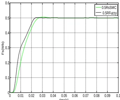
B. Stator resistance (𝑅𝑠)

The stator resistance changes with temperature, and it impacts the stator flux dynamics. Introducing a perturbation due to stator resistance error, the stator flux dynamics (34) is

= − 𝐹𝑠 +

Where 𝑅 𝑠 is the nominal stator resistance and 𝑅𝑠 is its actual value. We consider a maximum error in the

𝑅𝑠 −𝑅 𝑠| < 0.5 ×𝑅 𝑠 = 1.15. The corresponding model perturbation for the parameter values is 𝐺𝐹𝑠 = ×0.69 = 28.16. We choose the corrective control gain 𝑘𝐹𝑠 = 𝜂𝐹𝑠 + 𝐺𝐹𝑠 = 40 > 38.16. Since the torque dynamics is independent of the resistance error, we use the same value 𝑘𝑀 = 20, for similar dynamic performance. Simulation results in Fig. 4 show the stator flux and torque response for

resistance dynamic uncertainty. Note how the resistance error impact the flux response time, which is faster for lower resistances and due to larger gain. However, the steady state operation is ripple-free and robust with respect to Rs errors.

C. Rotor resistance (𝑅𝑟)

Rotor resistance changes with temperature. The prominent advantage of the proposed FBL is that the changes in Rr do not change the dynamics of stator flux and torque and do not affect the control. However, they do change the dynamics of the other two state variables (𝑅, 𝐹𝑟); this substantially impacts the speed estimate. Therefore, the rotor resistance errors are accounted for by speed errors discussed in section IV.A.

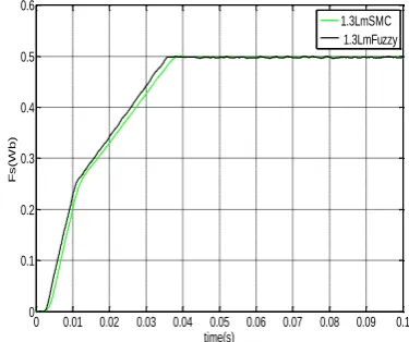
D. Magnetizing inductance (𝐿𝑚)

The magnetizing inductance deviate from its measured value due to magnetic saturation. Changes in the magnetizing inductance create changes in together the stator and rotor inductances. This has no effect on torque dynamics, but changes the stator flux dynamics (34), as follows:

= − 𝐹𝑠

+ (

̂

( ̂ )( ̂ ) ) wd

(37)

We consider a maximum change in the magnetizing

𝐿 𝑚 𝐿𝑚 𝐿 𝑚. We

𝐿 =

̂

( ̂ )( ̂ ) in (37) that depends on 𝐿𝑚. For

𝐿𝑚 = 0.7𝐿 𝑚 𝐿 = −0.42467, and for 𝐿𝑚 = 1.3𝐿 𝑚 we 𝐿 = 0.23176. For robust stability we

𝐿 |. The corresponding perturbation is 𝐺𝐹𝑠 = 2𝑅𝑅𝑠 × 0.42467 = 0.49. We use the gain 𝑘𝐹𝑠 = 12 > 10.49. Since the torque dynamics is independent of the magnetizing inductance, we use

𝑘𝑀 = 20.

Simulation results in Fig. 5 show the stator flux and

magnetizing inductance errors. Again, it is proved that SMC provide robust and ripple-free steady state performance. Overall, the largest gains can be used for all situations. All simulations are for the sensorless drive shown in Fig. 1. The proposed SMC design is based on the required dynamic response (𝜂𝑀, 𝜂𝐹𝑠) and the maximum uncertainty (𝐺𝑀, 𝐺𝐹𝑠). The dynamic response is application-dependent and is chosen by the designer. Equation (34) gives the maximum uncertainty caused by FBL. Given 𝜂 and 𝐺

for flux and torque, the designer chooses a sliding gain larger than 𝐺𝑀 + 𝜂𝑀 for the torque controller and better than 𝐺𝐹𝑠 + 𝜂𝐹𝑠 for the flux controller. This choice of the corrective control gains results in a robust and stable scheme that operates at the required speed while suppressing chattering. Comparing all simulation results, we terminate that larger gains result in a quicker and robust control, but can cause chatter if the increase in gain is excessive.

V.

interval of output state, so it is essential that this mathematical method is strictly distinguished from the more familiar logics, such as Boolean algebra.

Advantages of Fuzzy Controller over PI Controller

Usage of conventional control "PI", its reaction is not all that great for non-linear systems. The change is striking when controls with Fuzzy logic are utilized, acquiring a superior dynamic reaction from the system.

The PI controller requires exact direct numerical models, which are hard to get and may not give tasteful execution under parameter varieties, load unsettling powers, and so forth. As of late, Fuzzy Logic Controllers (FLCs) have been presented in different applications and have been utilized as a part of the power devices field. The benefits of fuzzy logic controllers over ordinary PI controllers are that they needn't bother with a precise scientific model, Can work with uncertain information sources and can deal with non-linearities and are more dynamic than traditional PI controllers.

VI.

Fig 3: Simulation results for SMC and FBL for proposed and extinction with +30% Lm errors, at

startup, torque Te s.

Fig4: Simulation results for SMC and FBL for proposed and extinction with -30% Lm errors, at startup, torque

Te s.

0 0.01 0.02 0.03 0.04 0.05 0.06 0.07 0.08 0.09 0.1

0 0.5 1 1.5 2 2.5 3 3.5 4 4.5 5

T

e

(N

m

)

time(s)

1.3LmSMC 1.3LmFuzzy

0 0.01 0.02 0.03 0.04 0.05 0.06 0.07 0.08 0.09 0.1

0 0.1 0.2 0.3 0.4 0.5 0.6

F

s(

W

b

)

time(s)

1.3LmSMC 1.3LmFuzzy

0 0.01 0.02 0.03 0.04 0.05 0.06 0.07 0.08 0.09 0.1

0 0.5 1 1.5 2 2.5 3 3.5 4 4.5 5

T

e

(N

m

)

time(s)

0.7LmSMC 0.7LmFuzzy

0 0.01 0.02 0.03 0.04 0.05 0.06 0.07 0.08 0.09 0.1

0 0.1 0.2 0.3 0.4 0.5 0.6

F

s(

W

b

)

time(s)

Fig 5: Simulation results for SMC and FBL for proposed and extinction with +50% Rs errors, at

startup, torque Te s.

Fig 6: Simulation results for SMC and FBL for proposed and extinction with -50% Rs errors, at

startup, torque Te s.

Fig 7: Simulation results for SMC and FBL for proposed and extinction with -10 rad/s speed errors, at

startup, torque Te s.

0 0.01 0.02 0.03 0.04 0.05 0.06 0.07 0.08 0.09 0.1

0 0.5 1 1.5 2 2.5 3 3.5 4 4.5 5

T

e

(N

m

)

time(s)

1.5RsSMC 1.5RsFuzzy

0 0.01 0.02 0.03 0.04 0.05 0.06 0.07 0.08 0.09 0.1

0 0.1 0.2 0.3 0.4 0.5

F

s

(

Wb

)

Time(s)

1.5RsSMC 1.5RsFuzzy

0 0.01 0.02 0.03 0.04 0.05 0.06 0.07 0.08 0.09 0.1

0 0.5 1 1.5 2 2.5 3 3.5 4 4.5 5

T

e

(N

m

)

time(s)

0.5RsSMC 0.5RFuzzy

0 0.01 0.02 0.03 0.04 0.05 0.06 0.07 0.08 0.09 0.1

0 0.1 0.2 0.3 0.4 0.5 0.6

F

s(

W

b

)

time(s)

0.5RsSMC 0.5RFuzzy

0 0.01 0.02 0.03 0.04 0.05 0.06 0.07 0.08 0.09 0.1 0

0.5 1 1.5 2 2.5 3 3.5 4 4.5 5

T

e

(

N

m

)

time(s)

-10%SMC -10%Fuzzy

0 0.01 0.02 0.03 0.04 0.05 0.06 0.07 0.08 0.09 0.1

0 0.1 0.2 0.3 0.4 0.5 0.6

F

s(

W

b

)

time(s)

Fig 8: Simulation results for SMC and FBL for proposed and extinction with +10 rad/s speed errors,

at startup, torque Te s.

(a)

(b)

Fig 9: Torque response to 4.5 Nm step command for proposed and extinction with (a) PI controllers (Linear DTC) and (b) PI controllers and FBL. Startup

from standstill.

(a)

(b)

Fig 10: Stator (blue) and rotor (red) flux magnitude control at startup, for proposed and extinction with (a)

PI controllers (Linear DTC) and (b) PI controllers and FBL.

0 0.01 0.02 0.03 0.04 0.05 0.06 0.07 0.08 0.09 0.1

0 0.5 1 1.5 2 2.5 3 3.5 4 4.5 5

T

e

(N

m

)

time(s)

+10%SMc +10%Fuzzy

0 0.01 0.02 0.03 0.04 0.05 0.06 0.07 0.08 0.09 0.1

0 0.1 0.2 0.3 0.4 0.5 0.6

F

s(

W

b

)

time(s)

+10%SMc +10%Fuzzy

0 0.005 0.01 0.015 0.02 0.025

-1 0 1 2 3 4 5

Time(s)

T

e

(

N

m

)

Electromagnetic Torque

0 0.005 0.01 0.015 0.02 0.025

-1 0 1 2 3 4 5

Time(s)

T

e

(

N

m

)

Electromagnetic Torque

0 0.01 0.02 0.03 0.04 0.05 0.06 0.07 0.08 0.09 0.1

-0.1 0 0.1 0.2 0.3 0.4 0.5 0.6

Time

S

ta

to

r

fl

u

x

0 0.01 0.02 0.03 0.04 0.05 0.06 0.07 0.08 0.09 0.1 -0.1

0 0.1 0.2 0.3 0.4 0.5 0.6

Time

S

ta

to

r

F

lu

(a)

(b)

fig 11: Torque transients for startup from standstill with feedback linearization and SMC (a) torque, (b)

stator and rotor flux magnitudes.

fig 12: Stator (blue) and rotor (red) flux magnitude response to 0.5 Wb step command for proposed and

extinction with feedback linearization and SMC, at standstill.

VII.

This paper proposes another design advance which incorporates Feedback linearization and Fuzzy logic controller with a DTC drive. This novel agreement in light of torque-flux linearization creates an automatic linear model of the IM, with torque and flux as decoupled state factors. For the linear IM show, the controller-observer partition guideline holds if estimation errors are little, which permit the controller and observer to be autonomously designed.

Fuzzy logic controller direct torque and flux control gives robustness against parameter uncertainties and their dynamics, as demonstrated by the correlation with a linear controller. The chattering related with sliding mode operation is disposed of by the corresponding controller utilized inside the limit layer. The drive has a similar quick and robust reaction, as a regular DTC drive and totally disposes of the torque and flux swell. Generally speaking, the arrangement consolidates the benefits of ordinary and linear DTC. These favorable circumstances are because of the sliding mode controller and the linearization which decouples the torque and stator flux extent.

VIII.

REFERENCES

1. I Takahashi, T. Noguchi, "A New Quick Response and High Efficiency Control Strategy of an Induction Motor," Rec. IEEE IAS, 1985 Annual Meeting, pp. 495-502, 1995.

2. G Buja, M.P. Kazmierkowski, "Direct torque control of PWM inverter-feed ac motors - A survey," IEEE Trans. Industrial Electronics, vol. 51, no. 4, Aug. 2004, pp. 744-757.

3. Y-S. Lai, W.-K. Wang, Y-C. Chen, "Novel switching techniques for reducing the speed ripple

0 0.005 0.01 0.015 0.02 0.025

-1 0 1 2 3 4 5

Time

T

e

(

N

m

)

Electromagnetic Torque

0.050 0.055 0.06 0.065 0.07 0.075 0.08 0.085 0.09 0.095 0.1

0.1 0.2 0.3 0.4 0.5 0.6

Time

S

ta

to

r

fl

u

x

0 0.005 0.01 0.015 0.02 0.025

-1 0 1 2 3 4 5

Time(s)

T

e

(

N

-m

)

Electromagnetic Torque

0.050 0.055 0.06 0.065 0.07 0.075 0.08 0.085 0.09 0.095 0.1

0.1 0.2 0.3 0.4 0.5 0.6

Time

S

ta

to

r

F

lu

of ac drives with direct torque control," IEEE Trans. Industrial Electronics, vol. 51, no. 4, Aug. 2004, pp. 768-775.

4. C Lascu, A.M. Trzynadlowski, "A sensorless hybrid DTC drive for high volume low-cost applications," IEEE Trans. Industrial Electronics, vol. 51, no. 5, Oct. 2004, pp. 1048-1055.

5. C Lascu, I. Boldea, F. Blaabjerg, "Variable-Structure Direct Torque Control A Class of Fast and Robust Controllers for Induction Machine Drives," IEEE Trans. Industrial Electronics, vol. 51, no. 4, Aug. 2004, pp.785-792.

6. MP. Kazmierkowski, D. Sobczuk, "High performance induction motor control via feedback linearization," Proc. IEEE ISIE-95, vol. 2, pp. 633-638, July 1995.

7. MP. Kazmierkowski, D. Sobczuk, "Sliding mode feedback linearization of PWM inverter fed induction motor," Proc. IEEE IECON 1996, vol. 1, pp, 244-249, Aug. 1996.

8. TK. Boukas, T.G. Habetler, "High-performance induction motor speed control using exact feedback linearization with state and state derivative feedback," IEEE Trans. Power Electronics, vol. 19, no. 4, July 2004, pp. 1022-1028.

9. D Sobczuk, M. Malinowski, "Feedback linearization control of inverter fed induction motor with sliding mode speed and flux observers," IEEE IECON 2006, pp. 1299-1304. 10. G. Luckjiff, I. Wallace, D. Divan, "Feedback

linearization of current regulated induction motors," IEEE PESC 2001, pp. 1173-1178.

11. John Chiasson, Modeling and high-performance control of electric machines, John Wiley and Sons Inc., 2005.