www.nat-hazards-earth-syst-sci.net/10/1085/2010/ doi:10.5194/nhess-10-1085-2010
© Author(s) 2010. CC Attribution 3.0 License.
and Earth
System Sciences
A new multi-sensor approach to simulation assisted tsunami
early warning
J. Behrens1,*, A. Androsov1, A. Y. Babeyko2, S. Harig1, F. Klaschka1, and L. Mentrup1,**
1Alfred Wegener Institute for Polar and Marine Research, Bremerhaven, Germany 2GFZ German Research Centre for Geosciences, Potsdam, Germany
*now at: University of Hamburg, KlimaCampus, Hamburg, Germany **now at: GCN Consulting GmbH, Bregenz, Austria
Received: 22 January 2010 – Revised: 3 May 2010 – Accepted: 11 May 2010 – Published: 7 June 2010
Abstract. A new tsunami forecasting method for near-field tsunami warning is presented. This method is applied in the German-Indonesian Tsunami Early Warning System, as part of the Indonesian Tsunami Warning Center in Jakarta, In-donesia. The method employs a rigorous approach to min-imize uncertainty in the assessment of tsunami hazard in the near-field. Multiple independent sensors are evaluated simultaneously in order to achieve an accurate estimation of coastal arrival times and wave heights within very short time after a submarine earthquake event. The method is validated employing a synthetic (simulated) tsunami event, and in hindcasting the minor tsunami following the Padang 30 September 2009 earthquake.
1 Introduction
The 2004 Great Andaman-Sumatra Tsunami spawned a large number of efforts to establish tsunami early warning capac-ities, to perform tsunami research, and to conduct mitiga-tion measures. Indonesia received a major contribumitiga-tion from the German Federal Government, which led to the devel-opment, installation and implementation of a new tsunami early warning system (TEWS) in Jakarta. The German-Indonesian Tsunami Early Warning System (GITEWS) de-velopment consortium consists of several large research lab-oratories and university partners in Germany and a number of research and government agencies in Indonesia (Rudloff et al., 2009). The GITEWS system is part of the Indonesian Tsunami Early Warning System (InaTEWS) at the Agency for Meteorology, Climatology and Geophysics (BMKG) in Jakarta. One of the design guidelines for the GITEWS
sys-Correspondence to: J. Behrens ([email protected])
tem was to enable the Indonesian authorities to give pre-cise, localized warning information after only a few minutes (definitely less than 10 min), since many tsunami sources are very close to the Indian Ocean coast of the Indonesian archipelago.
A key to precise short term information under the con-dition of high uncertainty in the first few moments after an earthquake is the utilization of multiple sensor information and synthesis of this information by means of advanced sim-ulation.
1.1 A review of current approaches
In spite of the large number of tsunamis that hit the Indone-sian coasts, until 2004 no dedicated operational TEWS was established in or around the concerned area. The two best es-tablished and long-time operational systems are maintained by the United States (with two sites at the Pacific Tsunami Warning Center, PTWC; and the West Coast and Alaska Tsunami Warning Center WCATWC), and by Japan (at Japan Meteorological Agency, JMA). These two systems follow very distinct approaches to tsunami early warning. While the JMA system faces a similar situation as InaTEWS, i.e. sources very close to the coast with little time for effective warning, the PTWC system is designed to give accurate in-formation, including inundation forecasts for densely pop-ulated areas on US territory, mostly far from the tsunami sources (Lautenbacher, 2005).
to yield wave heights at control points in 50 m water depth close to the coast. From these control points, using heuris-tic formulae (Green’s law) coastal wave heights are derived and used for warning level information. This approach gives a relatively large number of false positive warnings, since the estimation of the tsunami source is only based on pri-mary seismic parameters like location, magnitude and depth. However, the rationale behind this approach is to issue po-tential hazard information quickly and to verify (or falsify) the warning based on wave gauge measurements and give cancellation information as soon as possible. The system has been operational and effective for almost 10 years.
In contrast to this approach, PTWC relies heavily on tsunameter (deep ocean assessment and reporting on tsunamis, DART) measurements, installed approximately half an hour travel time from potential sources. A number of pre-computed unit sources with linear wave propagation scenarios is linearly combined, based on earthquake parame-ters and – when available – tsunameter readings, evaluated by a linear inversion procedure (Wei et al., 2008). The result is used for travel time information and preliminary wave height information, as well as initial condition for local real-time inundation simulations for certain areas of interest. From its design it is obvious that this approach intends to trade re-sponse time for better accuracy.
Several other approaches, including the formerly used sys-tem of BMKG in Indonesia use similar techniques or mix-tures of the above two. Many even simpler systems rely on just a decision matrix for tsunami early warning and do not even give localized warnings. The Indian Ocean tsunami warning system operated by the Indian National Center for Ocean Information Services (INCOIS) resembles the PTWC system to some extend, without using the real-time inunda-tion models. The Australian System jointly operated by Bu-reau of Meteorology (BoM) and Geoscience Australia (GA) is also similar, but renounces to use an inversion of tsuname-ter data (Greenslade et al., 2007).
1.2 Caveats and ideas
From the above description of current tsunami warning ap-proaches we can defer two insights. Currently, one can ob-tain very fast but inaccurate warning information. On the other hand, frequent false positive warnings render a warning system useless when end-users start to mistrust the alert. If accurate information is required, then time is needed for in-version and online computations. However, due to the short time between rupture and first wave arrival at the coast, for near-field tsunami warning there is no choice to rely on the lengthy inversion procedure so far employed in TEWS.
Time is one problem of near-field tsunami warning. An other problem is high sensitivity against the source mech-anism. While in the far-field case, a source can be de-scribed by primary seismic parameters such as magnitude, epicenter and directivity (Okal, 1988; Gica et al., 2007),
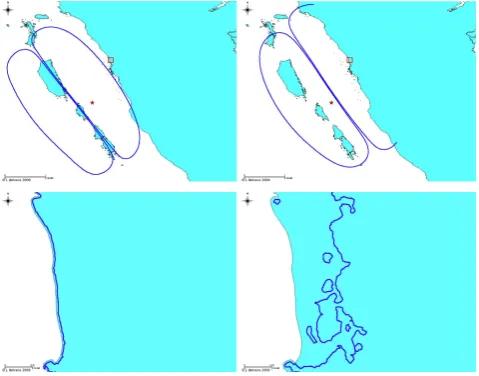
reli-Fig. 1. Top: two hypothetical tsunami sources corresponding to the same magnitude (Mw=8.5) and epicenter shown by a star. The
centroid of the scenario on the left lies some 50 km further west. Bottom: inundation area corresponding to the two different source models off Padang (zoomed area depicted as square in upper panels) showing that inundation in the near-field case sensitively depends on details of the slip distribution.
able tsunami prediction in the near-field requires much more detailed source characterization including fault geometry, ex-act position, orientation and heterogeneous slip distribution (Geist and Dmowska, 1999; Geist, 2002). Moreover, pecu-liarities of the off-shore local bathymetry become extremely important as well (see e.g. the difference in the December 2004 Tsunami and the March 2005 earthquake in Geist et al., 2006). An example is given in Fig. 1. The two hy-pothetic sources have the same epicenter off-shore Padang (marked with a star), same magnitude and direction, but their centroids, i.e., positions of maximal slip, lie some 50 km apart from each other. Additionally, bathymetry character-istics off-shore Padang (Mentawai islands) introduce very strong non-linearity to the tsunami propagation. Resulting inundations differ dramatically for the two scenarios. Thus, false positive warning would lead to major evacuation efforts, causing a lot of collateral damage without any inundation. On the other hand, a false negative would cause no warning with half the city inundated.
The basic idea of the new GITEWS approach is to use more than just the seismic and far field tsunameter informa-tion in order to reduce uncertainty on the tsunami source and derive an accurate forecast in short time. In particular, real-time GPS measurements of the earth crust displacement and wave gauge information (and here most prominently arrival time information) can beneficially be used in this context (Sobolev et al., 2007).
means to solve the inversion problem of tsunami early warn-ing:
Given measurements, what is the tsunami wave situation, and how will it evolve in the future?
Analog methods have been used in meteorology for quite some time, and are still in use for hurricane track forecast (e.g. Hope and Neumann, 1970). In strongly nonlinear dy-namics, analog forecast methods have been shown to be in-appropriate. But in tsunami forecasting the general wave propagation behavior is predominantly linear, allowing for a representer method to be valid. The strongly non-linear near shore wave interaction (note that this is not the general wave propagation) prevents the superposition of waves (or linear combination of scenarios as performed in the far-field case), thus giving an additional argument for using an analog method, which provides a best matching (single) representer. By means of combining several independent indications of a tsunami phenomenon, i.e. seismic information, co-seismic crust deformation measurements, and direct wave measure-ments by deep ocean and coastal gauges, uncertainty on the rupture can be reduced to give more accurate forecasts. 1.3 Outline of presentation
This article describes the principles of uncertainty reduction by independent sensor information for precise early warning information. The main ingredients for this approach are a well validated and accurate mathematical simulation model for the rupture source mechanism and tsunami wave prop-agation and inundation; a multi-sensor matching approach, based on well-behaved distance norms; a model for uncer-tainty propagation and handling during the forecast process; and an efficient implementation of these methods.
In the following section, we will develop a model for deal-ing with uncertainty. This is a simplified approach, which is aiming at operational efficiency and ease of use, even in an automatized system. Section 3 addresses the types and utilization of diverse sensors, including the derivation of a multi-sensor mismatch norm for measuring the distance be-tween reality and a pre-computed scenario. Section 4 gives a brief overview of how to implement the previously described methods in an operational environment, adhering to mod-ern system design standards. Results are presented based on a simulated tsunami events as well as a real event of 30 September 2009 in Sect. 5, before we draw conclusions.
2 Dealing with uncertainty
The key to accurate near-field tsunami warning is uncer-tainty. The problem to be solved can be formulated:
Given a set of uncertain data, derive a forecast, which sensitively depends on the given data.
This question has to be formulated in mathematical terms.
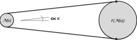
Fig. 2. Simple model for uncertainty propagation. The balls repre-sent uncertainty regions.
2.1 A model for uncertainty propagation
To start the mathematical formulation, we can write a fore-cast functional
F:x7→y=F (x); x∈ {Data},y∈ {Forecasts}. (1)
F maps given data (e.g. measured earthquake parameters) to a forecast (e.g. wave heights at coastal points of interest).
In order to take account for the uncertainty, we will con-sider a set of possible (uncertain) input data. F then acts on this set and generates a set of corresponding output val-ues (i.e. forecasts). Let us denote byXthe space of possible input data,xa member of that set, representing the theoreti-cal exact measurement,θxthe tolerance or uncertainty radius
(aroundx). In other words we have a subset
N(x)=Nθx(x):= {ξ∈X: kξ−xk ≤θx}, (2)
containing all possible inputs, under the uncertainty con-straint.
In order to assess the influence of the input uncertainty on the forecast, we need to apply the forecast functional on all elements ofN(x). Under reasonable assumptions on the regularity ofF we can formulate the following statement:
kN(x)k< θx⇒ kF (N(x))k< κ·θx, (3)
wherekN(x)kdenotes the diameter of the set, orθxdenotes
the maximum distance of an uncertain input from the the-oretical exact measurement. Note thatF (N(x))is a set of forecasts. Equation (3) states that if the input data is within a given uncertainty range, then the forecast uncertainty is am-plified by a factor 1≤κ≤ ∞(see Fig. 2). κ represents the sensitivity of the problem. If κ1 the forecast can vary greatly even for small input perturbations. Ifκ= ∞, no fore-cast is possible, the problem is ill posed. Therefore, we will assume thatκ <∞.
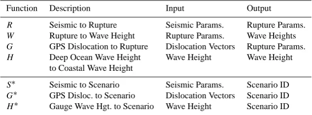
Table 1. Common forecast functionals in tsunami forecasting.
Function Description Input Output
R Seismic to Rupture Seismic Params. Rupture Params.
W Rupture to Wave Height Rupture Params. Wave Heights
G GPS Dislocation to Rupture Dislocation Vectors Rupture Params.
H Deep Ocean Wave Height Wave Height Wave Height to Coastal Wave Height
S∗ Seismic to Scenario Seismic Params. Scenario ID
G∗ GPS Disloc. to Scenario Dislocation Vectors Scenario ID
H∗ Gauge Wave Hgt. to Scenario Wave Height Scenario ID
IfFis not just one function but a composition of functions, we have the following relation. LetF=W◦R, whereW and
R are individual forecast functionals. We can think of the sequence:Rmaps seismic observations to a rupture forecast, which in turn is mapped byW to a forecast on wave heights. Thus, let
R :X→Y,x7→y=R(x), W :Y→Z,y7→z=W (y),
withx∈X input for R, y∈Y forecast of R and input to
W, and z∈Z the forecast (output) ofW. Let furthermore
kN(x)k ≤θxbe the uncertainty range inX,kN(y)k ≤θythe
uncertainty range inY. Since the two functionals are com-posed, we have thatθy≤κR·θx. Therefore, the uncertainty
range in the composed result
W◦R:X→Z;x7→z=(W◦R)(x) (4) takes the form
kN[(W◦R)(x)]k = kN(z)k ≤θz≤κWθy≤κWκRθx. (5)
Thus, in a composition, the initial uncertainty is amplified multiple times.
2.2 Applying the uncertainty model to tsunami warning
We have to define the forecast functionals now. There are several common ways to forecast tsunamis and to utilize these forecasts in TEWS. A straightforward and simple way is to take seismic parameters as an input and derive a warn-ing level by means of a decision matrix. The functional thus maps seismic parameters to warning level:
F : epicenterlat,epicenterlon,magnitude,depth −→ −→ {tsunami advisory,tsunami watch,...}
It is not important to consider the internal mechanics of the mapping functional. This forecast functional is discrete, therefore the theory with regularity assumptions is hard to apply. In any case, the uncertainty amplification also holds
and in particular the uncertainty amplification factor κ can increase drastically when the sensor regime is close to thresh-old values determining the change from one warning level to the other. Other more common forecast functionals are listed in the upper part of Table 1.
In most approaches to tsunami early warning a combina-tion of seismic informacombina-tion and simulacombina-tion is used. There-fore, a combination of functionalsR andW from Table 1 is used. In other words, the forecast functionalF is a composi-tionF=W◦R.
In the case of near-field tsunamis, both forecast function-als are sensitive to input uncertainty. The sensitivity factors
κRandκWcan be derived by simple Monte-Carlo style
sensi-tivity analysis (Mentrup et al., 2007). In this case, each factor is large, leading to an almost useless forecast, when combin-ing these two forecasts (i.e. multiplycombin-ing two large factors). This is the reason for so many false positive warnings in tra-ditional near-field tsunami warning systems.
In the far-field tsunami case, at leastκWis small, i.e. sen-sitivity on the exact source description for wave height fore-casts is not high. Therefore, this case works much better with purely seismic source information. In the PTWC system, the uncertainty factorκRis also minimized, by not only
consider-ing seismic information for a computation of the rupture, but also using tsunameter data for reducing the uncertainty on the exact rupture parameters. Therefore, that system works very precisely to the expense of lengthened time to acquire the necessary data.
3 Multiple sensor systems
3.1 The principle of uncertainty reduction with multiple sensors
The main difference of the GITEWS approach is that no compositions (resulting in uncertainty magnification) are used. All the forecast functionals have one and the same goal: to select a tsunami scenario that represents reality. In particular, we have the forecast functionals described in the lower part of Table 1. Since they all map into the same image space, they can be combined, as shown in this paragraph.
Of course, GITEWS also uses wave height indicators to yield forecast information, which in turn are derived from the scenarios. But it should be noted that the different sen-sors all describe the same complex system in reality, which is represented in the scenarios. Each scenario consists of a tsunami source model as well as a wave propagation and in-undation model. It should further be noted that this approach only works, if the models are well validated and represent physical processes of the real earth system.
We consider the GITEWS forecast functionals
S∗:S→I, s7→S∗(s)=i, G∗:G→I, g7→G∗(g)=i, H∗:H→I, h7→H∗(h)=i,
wheres,g, andh are inputs from seismic, GPS, and wave height sensor systems, respectively;iis in the set of scenario IDs. LetN(s), N(g),N(h) be the uncertainty regions in the seismic parameters, the GPS dislocation vectors, and the wave height measurements, respectively.
We assumekN(s)k ≤θS∗,kN(g)k ≤θG∗, andkN(h)k ≤ θH∗withθS∗6=θG∗6=θH∗, which means the different sensor
systems have different accuracy levels (uncertainties). With
kIS∗k = kS∗(N(s))k ≤κS∗θS∗, kIG∗k = kG∗(N(g))k ≤ κG∗θG∗, and kIH∗k = kH∗(N(h))k ≤κH∗θH∗ respectively,
we further assumeκS∗6=κG∗6=κH∗, i.e. each of the
differ-ent forecast functionals in the GITEWS system may have a different sensitivity.
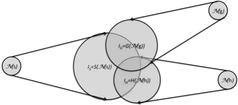
Since all functionals map to the same space independently, they can be combined (instead of being composed). Since all three functionals map into the set of scenario IDs, the com-bined result is the set of IDs, which is contained in each of the imagesIS∗, IG∗, IH∗, i.e. contained in the intersection IS∗∩IG∗∩IH∗(see Fig. 3).
Thus, uncertainty is greatly reduced by the combined multi-sensor approach. In fact, each additional independent sensor system that monitors the same physical phenomenon, and can be simulated in terms of the same integrated scenario approach, can reduce the uncertainty.
Note that Fig. 3 points to an important prerequisite for this approach to work: The scenarios need to represent all pos-sible configurations in reality and need to be validated to match with real sensor data, since otherwise we might find ourselves in the situation of an empty intersection. We will
Fig. 3. Combination of multiple sensors and corresponding uncer-tainty propagation. The intersection of the image areas marks the set of possible results of a combined matching.
see, however, that this is a theoretical statement. The im-plementation of the GITEWS system tolerates less rigorous assumptions.
In the warning process, there will be different states of the sensor network. At an early state only a fraction of the sen-sors may have received a signal. Thus not all of the map-pings can be combined at this time. At a later state, the data situation may have improved and additional information leads to reduced uncertainty. The theory, developed above, assumes a complete picture of the situation. Again in the implemented system, this is not a prerequisite.
Note further that we will not use the outlined theory for matching pre-computed scenarios to given data. The theory developed so far justifies the multi-sensor approach in terms of uncertainty reduction. We will now develop the multi-sensor matching procedure.
3.2 Independent indicators – description of sensor systems and scenarios
We saw in the previous subsection that we need to combine independent sensor systems in order to reduce uncertainty in the forecast process. In our approach, three different inde-pendent systems are considered:
– the seismic system, giving earthquake location, magni-tude and depth;
– the real-time GPS system, giving 3D dislocation vectors at sensor positions;
– the wave gauge system, giving arrival time and wave height time series at sensor positions.
location of the source. Finally, the GPS signal of a smaller (still tsunamogenic) earthquake may be too weak to be de-tected. In this case, however, the source is small enough to be accurately characterized by the seismic parameters. If, on the other hand, the rupture area is so large that the seismic pa-rameters are ambiguous with regard to the exact location and extent of the uplift, then the GPS signal will be significant enough to contribute to an uncertainty reduction.
If we think of the earth system in a holistic way, then the above mentioned sensor systems are of course not inde-pendent. A release of a locking situation causes an earth-quake and is responsible for the uplift area, which in turn is uniquely determining the hydrologic wave behavior. How-ever, in terms of indicators of a phenomenon and in terms of uncertainty, these aspects of a natural phenomenon are inde-pendent. They all shed light on the phenomenon from dif-ferent angles of perspective, and in particular with difdif-ferent (independent) types of measurements.
On the other side, our scenarios also contain models, which yield synthetic representations of the above sensor systems. Our source model relates a certain initial uplift function to certain seismic parameters and GPS disloca-tion vectors. The wave propagadisloca-tion and inundadisloca-tion model adds information on corresponding wave heights and arrival times.
3.3 Utilizing sensor systems – from measurement to forecast
In order to use the mentioned sensor systems for the forecast of tsunami hazard, we will match given data to scenario data. In contrast to the theory, we will not use explicit forecast mappings, but will try to define a distance measure from the truth. For each scenario we will then have a value for its distance to the true state of the tsunami event.
Before we can start with defining a generalized distance measure, we will look for individual distances. This is rel-atively straight forward for most of the data types, present in the system. Table 2 lists the data types and correspond-ing distance definitions (norms). The only critical distance metrics are for magnitude and gauge time series. We use either a direct comparison of the moment magnitude val-ues, or a comparison of the seismic moments. For time se-ries comparison we use a simple 1-norm approach. These choices are still to be validated in the real warning center en-vironment.
The given individual norms are extended by an uncer-tainty model. We start with an example. In our scenar-ios, we assume that the earthquake epicenter is located in the geometrical center of the rupture area. In reality this is not generally the case. In fact, the epicenter usually lies somewhere in the rupture area. Thus, the reported epicen-ter may correspond to several precomputed scenarios – those with rupture areas covering the reported location. We do not
Table 2. Data types, sensor systems and individual norms in the GITEWS system. Indexed values represent scenario data.
Sensor Data type Distance norm
system
Seismic epicenter locationx=(x, y) dloc= kx−xik2 epicenter depthD dD= |D−Di| moment magnitudeMw dM= |Mw−Mwi|, or
dM= |mo(Mw)−mo(Mwi)|, where mo(µ)=10(3/2)µ+9.1 GPS dislocation vectorx=(x, y, z) dGPS= kx−xik2
Gauge arrival timet dT= |t−ti| time series t=(t1,...,tN) dTS= kt−tik1
match the exact value of the earthquake location, but the lo-cation and an uncertainty range. In mathematical terms:
dloc=maxkx−xik2− |U|,0, (6) whereU is the radius of an uncertainty area. For each data type an individual uncertainty radius may be used. For ex-ample, the uncertainty radius for the epicenter is initially es-timated according to the scaling laws for the rupture dimen-sions (Wells and Coppersmith, 1994). We apply the same theory to all the different available data types. Therefore, uncertainty radii are parameters for optimization.
The uncertainty radii make the system robust against noise in the data. Note that the multi-sensor approach (in which all the different data – even though perturbed – need to repre-sent a physically consistent real event) stabilizes the selec-tion. Even if the data is noisy (but not too noisy to hide any signal), the multi-sensor approach allows for reduction of un-certainty.
After having introduced individual norms and a sensitivity model in the matching process, we now need to harmonize the data. First of all, the different norms need to be compa-rable. In order to achieve that, we will normalize the data, i.e. we will map them to the unit interval. Note that we are not interested in the actual values, but we are interested in the distances. Additionally, we are interested to distinguish small differences, while a large distance does not need to be differentiated. Therefore, we choose a non-linear mapping in the following way:
scal(d)= 2
πarctan(ν·d) , (7)
After these manipulations we are now in the situation that we can measure distances (between real sensor readings and scenario data) for individual data types and sensors. These distances are comparable, since they are all mapped to the unit interval. Additionally, they consider uncertainty and noise in the measurement data. It will be the aim of the fol-lowing subsection to combine the individual distance metrics to a generalized norm.
3.4 Combining independent sensor systems
In order to combine individual distance norms to a compound a simple weighted sum approach is used. The seismic system delivers data already in aggregated form. Individual sensors (i.e. seismometers) are not directly connected to the simula-tion system. But for other systems, we need to combine in-dividual sensors to sensor groups first. In order to be able to weigh different sensor systems individually, and not overem-phasize individual sensors, the following compound norms for the wave gauge and GPS systems are defined:
Dσ=
X
i=1:Mσ
wσidσi, (8)
where σ ∈ {GPS,T,TS} indicates the sensor system/data type. Here GPS indicates the real-time GPS dislocation vec-tors, T the arrival times, and TS the wave height time series at gauges (see Table 2). Moreover,Mσis the number of sensors
available in the sensor network, andwiσ are weights, defined by
ˆ
wiσ=
0, if the sensor is not available;
0.5,if the sensor is not reliable;
1, if the sensor is fully functional.
(9)
Then the weights are normalized (i.e.P
iwiσ=1) by
wiσ= ˆwiσ· X
i
ˆ
wiσ
!−1
. (10)
Note that sincedσi is a scaled distance norm with values in the unit interval [0, 1] and since thewiσ are normalized, the compound normDσ, defined in (8), has its values also in the
unit interval.
Now, by usingDloc=dloc, DD=dD, DM=dM(see
Ta-ble 2) and Eq. (8), we have defined distance norms for the six different available data types in the TEWS. It is our aim to combine these to a generalized distance. Again, this is achieved by using the weighted sum approach:
D= X
S∈{loc,D,M,GPS,T,TS}
WSDS, (11)
whereWSare normalized weights. We will callD the
mis-match. Note that the weights can be tuned. In our exper-iments we found that the mismatch is relatively insensitive to the fine tuning of weights. However, the weights give the
possibility to emphasize the relevance or reliability of cer-tain measurements over others. In our case, we will assign a larger weight to the direct (gauge) measurements of the wave, compared to the indirect indications of a tsunami (namely, the seismic information and the GPS information).
The mismatch value has several properties, which are im-portant to note. The mismatch lies in the unit interval. If data in a specific data type is missing, the corresponding weight is set to zero. A mismatch valueD=0 indicates a perfect match (within the uncertainty range) to given measurements. In other words, if D=0, then the corresponding scenario lies in the intersection of the combined forecast functionals as in Sect. 3.1. A large mismatch value (i.e. 0.5 and above) means little resemblance of the scenario to the measured si-tuation. With increasing availability of data types, the mis-match value can deteriorate (the absolute value grows). But this does not necessarily mean a worse correspondence to the real situation! We will elaborate on this in the following subsection. Note that the absolute value of the mismatch de-pends on a number of factors, including the tuned weights, the (tuned) uncertainty radii, etc. Therefore, it is not worth, considering the actual value, except for ordering the list of pre-computed scenarios for their matching quality.
3.5 Evaluating the mismatch value – reliability and skill
In order to gain insight into the behavior of the mismatch value, the following setting is considered. In a tsunami event, after a short time seismic information is available. A match-ing with pre-computed scenarios is performed and yields zero mismatch value for all those scenarios in the uncertainty range of the epicenter location and magnitude given. Af-ter some time, additional wave gauge information becomes available. Now, the mismatch value increases with a clear ranking among the scenarios. This can happen, if the earth-quake source is not among the pre-computed scenarios; in which case none of the scenarios lies exactly in the intersec-tion of the two forecast funcintersec-tionals. In spite of the fact that more information is available, the mismatch deteriorates – a counterintuitive behavior.
The reason for this behavior is that none of the pre-computed scenarios matches reality exactly. The best match-ing scenario might still be in the uncertainty range of the seismic system and taking those values for matching would still give a zero mismatch value. However, if only one of the gauges measures a different signal than present in the scenario, the mismatch becomes non-zero. So, in order to obtain a useful quantification of the suitability of a matching scenario for tsunami hazard forecasting, additional indicators are needed.
not available. At the same time, the weights used in the mis-match computation, in comparison with all possible values give an indication on the availability and therefore reliability of the data.
With this, we formally define the reliability index by
R=
P
i∈(available groups)Wi·
P
j∈(available sensors)w j i
P
i∈(all groups)Wi·
P
j∈(all sensors)w j i
. (12)
Note that since we normalized our weights, the denomina-tor is 1, therefore, only the numeradenomina-tor needs to be computed. Note further that 0≤R≤1. If R=0 then no sensors are available, therefore any matching result would be pure guess-ing and not reliable at all. If all sensors are available, i.e.
R=1, then we cannot do better in terms of sensor availabil-ity, the matching result is reliable. It does not mean that the mismatch is good, though.
Now, if we had scenarios of different quality, say some that include a model for the earth crust deformation and oth-ers that do not. Then the mismatch for those scenarios with less values to compare could be better than for those includ-ing the earth crust model (for the same argument as in the experiment of thought at the beginning of this subsection). In order to derive a quantitative means to distinguish these cases, we introduce the skill index, which is defined as the ra-tio of matched measurements over available measurements.
S=
P
i∈(used groups)Wi·
P
j∈(used sensors)w j i
P
i∈(available groups)Wi·
P
j∈(available sensors)w j i
=
P
i∈(used groups)Wi·
P
j∈(used sensors)w j i
R . (13)
Note that 0≤S≤1. IfS=1 all available data could be com-pared with scenario data, therefore the scenario has a high skill (usability).
It is important to notice that the reliability indexR is a quantification of uncertainty related to the available data, while the skill indexSis related to the matched scenario.
4 Implementation issues
In the previous sections a theoretical motivation and algo-rithm for the multi-sensor approach to tsunami early warning has been developed. It is now the aim to describe the imple-mentation of the system and the related supporting scenario software.
4.1 The need for an accurate model
From the theory it became clear that the multi-sensor ap-proach intends to reduce uncertainty in the forecasting pro-cess. Since this approach is combined with an analog
method, where the forecast relies on pre-computed scenar-ios, it will only work, if the scenarios are matching real sit-uations. The scenarios will, for example, contain a systemic bias, if the wave heights do not fit to the magnitude/location parameters from the seismic system. This sounds trivial, but the likelihood for inconsistencies grows with the number of physical processes/data types represented in the model.
In the GITEWS system, a coupled simulation software setup is utilized for the scenario generation. It consists of a source model (RuptGen), which interprets incoming seismic parameters and calculates initial wave profile as well as co-seismic 3-D surface dislocations at selected GPS-positions, and a hydrodynamic wave propagation and inundation model (TsunAWI). RuptGen has been developed at GFZ German Research Centre for Geosciences by Babeyko et al. (2010). It discretizes the 3-D Sunda subduction zone plate interface into numerous patches and employs Green’s functions tech-niques and seismic scaling laws to construct a finite-fault rupture and calculate corresponding co-seismic surface de-formations.
The operational tsunami wave propagation and inundation model TsunAWI is based on unstructured finite elements to allow for local refinement close to the coast and in priority ar-eas. Additionally, the unstructured triangular grid allows for locally accurate representation of complex boundaries (Harig et al., 2008). TsunAWI is fully validated along the line of Synolakis et al. (2008) for operational tsunami simulation systems (Androsov et al., 2008).
An inundation result for Padang/West Sumatra including the unstructured mesh outline, and a wave propagation snap-shot from TsunAWI are depicted in Fig. 4.
4.2 Open system architecture
In order to implement the methodology into a TEWS, and af-ter having computed a repository of scenarios, the data needs to be managed in an efficient way. Several important prereq-uisites need to be fulfilled. Time is an important issue. There-fore, one design goal is to compute a forecast within less than 10 s. Furthermore, automatic data management should be easily achievable. The simulation system (SIM) is part of a complete system architecture, in which the sensor systems, the communication infrastructure, the decision support sys-tem and the dissemination syssys-tem are key components (see Fig. 5).
Internally, the SIM is organized in the following functional units, depicted in Fig. 6:
Fig. 4. Detail of a grid and inundation flow depth in Padang, West Sumatra, Indonesia, used in the operational tsunami propagation and inundation model TsunAWI (left), and a typical propagation example for the Indian Ocean (right).
– Selection module: the selection module implements the matching logic, described in Sect. 3.
– Index database (IDB): in order to achieve performance, the scenarios are harvested for indexed data, i.e. the rel-evant data at sensor locations, some meta-data, and an identifier.
– Index database updater (IDU): the IDU is the harvester, which automatically retrieves indexed data from the scenarios.
– Post-processing unit (PPU): this unit consists of plugins for several pre- or post-processed visualization and data products. Currently all data output is transferred in SHP file format.
– Driver level (driver): in order to allow for diverse sce-nario data formats, a driver level hides the details of each scenario data format from the SIM internal data structures.
– Tsunami scenario repository (TSR): a large file system storing tsunami scenario raw data. It is necessary to store these, since each new sensor location necessitates the IDU to harvest all scenarios for the sensor data. The basic workflow in the system consists of two phases: the ingestion phase, and the selection phase. In the inges-tion phase, which is run preferably in idle times (or on a stand-by non-operational system), new scenarios or sensor locations are ingested, and data products are computed, upon request of the DSS. The DSS stores pre-computed maps for each scenario registered in the IDB for quick access in case of a tsunami event. In the selection phase, the DSS sends data messages to the SIM, corresponding to the current state of the sensor systems. The SIM takes these data messages to the selection unit and performs a matching, according to the
Fig. 5. Overview of the GITEWS system architecture as seen from the simulation system (SIM) perspective. Data are gathered by the sensor systems, passed through a data management unit (tsunami service bus) and evaluated, merged and visualized by the decision support system (DSS), before being disseminated.
Fig. 6. System architecture of the simulation system: input and out-put modules utilize the web processing service (WPS) and web no-tification service (WNS). The selection unit implements the multi-sensor selection mechanism, comparing measurements with in-dexed scenario data in the index data base (IDB), which in turn is filled by the index data base updater (IDU). IDU and post-processing unit (PPU) access data in the tsunami scenario repository (TSR) through a driver.
procedure outlined in Sect. 3. It thus returns a list of scenario identifiers, with corresponding mismatch values, reliability index and skill indices. The DSS then uses this information to derive a situation analysis and a corresponding warning bulletin proposal.
5 Results
In order to validate our approach, we first show a synthetic benchmark tsunami event, which was used extensively dur-ing the development phase of the system. Since the sys-tem is in operational testing since November 2008, one real life tsunami incident can be used for further evaluation, the 30 September 2009Mw=7.7 earthquake and minor tsunami
Fig. 7. Bechmark slip distribution (left) and sensor network (right). The two benchmark gauge locations are marked by a red pentagon, and the epicenter location by a red star. Orange triangles indicate GPS stations and blue circles represent the buoy locations.
5.1 An artificial benchmark experiment
The synthetic benchmark experiment has been derived in the following way: An independent group within the GITEWS consortium, computed a tsunami event for the area of Padang, taking a complex rupture (slip distribution is shown in Fig. 7, and follows that of the Bengkulu 12 Septem-ber 2007 event shifted closer to Padang). Correspond-ing GPS dislocation vectors (at the positions of the Suma-tran cGPS Array SuGAr network1), seismic parameters, and wave height values at two GITEWS buoy locations as well as at benchmark gauge locations in Padang and Bengkulu were given. Computations for these values were made by RuptGen for the GPS vectors and by an independent finite difference tsunami wave propagation model for the gauge values. The assumed sensor network is depicted in Fig. 7. The assumed earthquake has a moment magnitude of 8.0 (MW) and its
epi-center is located at (99.93◦E, 1.96◦S).
We perform several experiments. First, we show the re-sult of a matching with only the seismic parameters (epicen-ter location and magnitude) given. Since sensitivity of this forecast functional (see Sect. 2) is high, large uncertainty is present in this forecast. The list of possibly matching ios is derived by looking at the mismatch values. All scenar-ios are sorted with increasing mismatch value. It turns out that some of the scenarios get similar mismatch values and that certain plateaus are visible in the mismatch histogram (see Fig. 8). The list of scenarios is cut off, after the second such plateau, where the detection is based on evaluating the difference histogram.
1http://www.tectonics.caltech.edu/sumatra/sugar.html,
last access: 26 May 2010
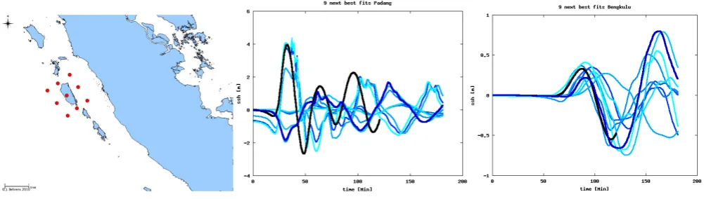
Figure 9 shows the locations of all those scenarios with epicenters in the uncertainty range of the seismic forecast functional (and the few more, which are in the mismatch list). This results in largely uncertain results for the forecasts in both benchmark regions. A decision maker in the warning center would still do a reasonable job for Padang, when tak-ing the worst case to forecast arrival time and wave height. However, in Bengkulu, the worst case forecast would largely overestimate the true effect of the tsunami. Note that out of the selected 32 possible scenarios, 22 have a mismatch value of zero. The remaining 10 have mismatch values between 0.0003 and 0.008. Reliability index is 0.22, and the skill is 1.0, since all scenarios can match all given data. In fact, since we can always match all measurements, all scenarios and ex-periments in this section have a skill 1.0.
Fig. 8. Mismatch histogram for the synthetic test case with approximately 220 pre-computed scenarios (left). The difference plot (right) shows the difference of mismatch values of predecessor scenario to following scenario. Peaks show the location, where a next “plateau level” in the mismatch list is reached. The list is cut off after the second significant peak, where the horizontal line indicates the threshold value for
significant.
Fig. 9. Benchmark experiment with given seismic parameters. The locations of matching scenarios (left) and the corresponding mareograms in comparison with the benchmark gauge time series for Padang (center) and Bengkulu (right) are shown. Dark color indicates small mismatch, light color larger mismatch.
Fig. 11. Benchmark experiment with given seismic parameters, arrival times and wave height time series at buoy locations (see Fig. 9 for description of the three panels).
Fig. 12. Benchmark experiment with given seismic parameters and GPS dislocation vectors (see Fig. 9 for description of the three panels).
Adding a time series comparison at the buoy locations (and here, we compare only those few measurements, which are available up to 5 min after the rupture, and we use a sam-pling rate of only 1 min), we can further reduce the uncer-tainty. Only three scenarios are left in the uncertainty range (see Fig. 11). Two of them (in dark blue) represent the best matching scenarios in the repository to the “true” event. A decision maker can now give a precise warning with great confidence. The reliability in this case is 0.66. From the three examples shown so far, we see that the reliability in-creases with the number of sensor readings available for the matching. Consequently, the uncertainty decreases, and the forecast becomes more accurate.
Note that none of the scenarios has zero mismatch value any longer. This is due to the fact that the complex rupture cannot be reproduced exactly by any scenario in the repos-itory. However, the best matches still give a very accurate resemblance with the “true” event. It should further be noted that this data coverage is a little unfair. In real life, the wave height time series at the buoys may not be so well behaved. In particular, since the buoys are located close to the sources, a superposition of seismic signals with water waves can oc-cur, which will possibly render the time series information uncertain.
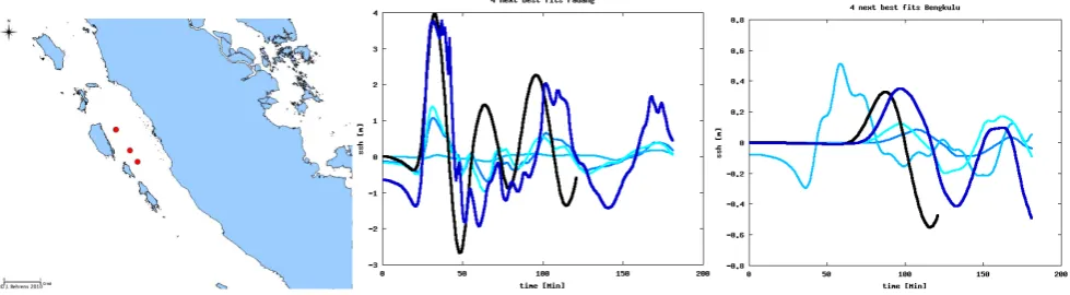
So, let us try to use the GPS signal instead. Starting from the seismic data set (epicenter location and magnitude), we add the GPS signals. In fact, only significant signals add any information, since the uncertainty here is in the range of 5 cm (every dislocation below that threshold is taken to be zero). This information reduces the uncertainty greatly, so that only three scenarios remain in the set of possibilities (Fig. 12). However, at least one unrealistic scenario cannot be ruled out just by adding GPS information. In spite of this, a deci-sion maker would give a much better warning with than with-out the additional GPS information: from maximum wave heights, rather correct warning levels would be derived. Only the arrival time for Bengkulu would be too conservative. The reliability for this case is 0.44. Data from real-time GPS-arrays are available in just a few minutes after the earthquake event, which makes this type of data very valuable for the near-field early warning (Sobolev et al., 2007).
Fig. 13. Benchmark experiment with given seismic parameters, wave arrival at buoys, and GPS dislocation vectors (see Fig. 9 for description of the three panels).
Table 3. Stages in the evaluation of the Padang earthquake.
Data set Timestamp Time after rupture Location Magnitude GPS used
1 10:18:11 UTC 2:05 min (0.944◦S, 99.511◦E) 7.5 no 2 10:19:48 UTC 3:39 min (0.905◦S, 99.629◦E) 8.3 no 3 10:21:10 UTC 5:02 min (0.958◦S, 99.563◦E) 8.3 yes 4 10:25:20 UTC 9:12 min (0.958◦S, 99.563◦E) 8.2 yes
5.2 Hindcasting the Padang earthquake and tsunami from 30 September 2009
On 30 September 2009, 10:16 UTC, a strong earthquake occurred with an epicenter location at (0.78◦S, 99.87◦E) and a moment magnitude Mw=7.7 (GFZ Potsdam, 2009).
The earthquake caused an official number of 1115 casualties in Padang and nearby communities (Antara News, 2009). Additionally, it triggered a minor tsunami. In contrast to JMA and PTWC, which act as interim regional tsunami watch providers in the Indian Ocean region, the Indonesian Tsunami Warning Center at BMKG issued no tsunami warn-ing. This was a correct assessment of the situation.
The multi-sensor selection simulation component of the InaTEWS/GITEWS system was not used for this assessment, since many of the non-seismic sensors were not yet avail-able, or did not deliver online sensor readings. In order to reconstruct and hindcast the event with the future capacity of the multi-sensor selection based simulation system, we look at the stages of the sensor system, listed in Table 3. GPS data were available from two sensor locations, in Se-blat (3.2◦S, 101.5995◦E) and Nias (1.3◦N, 97.57◦E). Both readings were insignificant, supporting the assumption of an earthquake with minor uplift and thus minor tsunami gener-ation. In addition, both stations are probably too far from the rupture area in this case.
Analysis of the seismic data suggests that this was not a typical mega-thrust type earthquake but was an intra-plate earthquake (Lange et al., 2009; Grijalva et al., 2009). Thus, the pre-computed scenarios do not have the chance to resem-ble the true situation exactly. However, it is the goal of this section to asses the suitability of the forecasts, in such a real-life situation.
The first seismic estimate of the situation was available af-ter approximately 2 min, and gave a reasonable (compared to the final seismic parameters) estimation of the basic seismic situation. The closest pre-computed scenario is depicted in Fig. 14. Its epicenter location (0.91◦S, 99.62◦E) is further to the West. In fact, one of the results of this event was the decision to extend the area of pre-computed scenarios further to the East. However, the warning levels, derived from this scenario would suggest no warning since the maximum wave heights along the coast close to Padang is everywhere below 0.5 m.
Fig. 14. Result of the selection after 2 min (data set 1). The red and blue line indicate the outline of the vertical sea bottom displacement (red – positive, blue – negative). The different measured epicen-ter locations with circle size indicating the magnitude are shown. Green points at the coast indicate no warning level (green – no warning, orange – tsunami warning, red – major tsunami warning), or maximum wave height lower than 0.5 m.
Fig. 15. Result of the selection after 3.6 min (data set 2), analogous to Fig. 14. The selected scenario corresponds to a magnitude 8.5 (Mw) earthquake, largely over-estimating the true event.
The GPS data in the third data set, do not really help to improve the situation. Since only two GPS stations deliver data, the reliability increases to a still very low value of 0.28. In this case, one of the stations delivers data below the rele-vance threshold. One station’s data just slightly exceeds the confidence interval of the GPS system, which at the time of the experiment was computed to be approximately 1.5 cm. However, it turns out in data set 4 that this value is caused by a temporary displacement or by atmospheric disturbances.
Fig. 16. Result of the selection after 5 min (data set 3), analogous to Fig. 14. An insignificant GPS signal spoils the selection solution, since now a scenario with a dislocated uplift area is selected. Its
Mw=8.2.
This faulty signal causes the selection system to suggest a scenario, for which the uplift area is far from the seismic system’s epicenter location. The forecast, however wrong, would suggest no tsunami warning (see Fig. 16). Since the seismic parameters do not indicate major dislocations at the GPS stations in the scenarios, a non-zero mismatch value of 0.0016 is now computed.
Finally, after approximately 9 min (data set 4) none of the two GPS stations report a significant signal. In other words, both station’s values do not exceed the confidence intervals and are therefore taken to be zero. In spite of the fact that these signals are of minor relevance, they are taken into ac-count in the matching process. Therefore, reliability is 0.28, as with data set 3. However, the matching is now again con-sistent with a mismatch value of 0.0. Since the seismic pa-rameters are still over-estimated, a scenario withMw 8.0 is
selected, yielding a warning level corresponding to “tsunami warning” (Fig. 17).
It turns out that for events with a magnitude of 7.5 and lower, it is paramount to do a proper seismic parameter esti-mation. GPS signals may be useful, if a dense enough GPS network is available. In the case of the Padang earthquake, the stations were too far from the rupture area to yield rele-vant information. In fact, it might be useful to filter tempo-rary dislocations, if unreasonable. The first data set, with its correct assessment of the seismic parameters, yields a realis-tic and accurate tsunami situation assessment. The selection depends sensitively on correct sensor readings.
Fig. 17. Result of the selection after 9 min (data set 4), analogous to Fig. 14. Due to the over-estimated seismic magnitude, the warning level derived from the matched scenario over-estimates the potential hazard.
6 Conclusions
A new near-field selection procedure for inverting the tsunami hazard situation from given online sensor measure-ments has been developed. The method is based on a rigor-ous uncertainty propagation and quantification model. The model not only motivates a multiple sensor evaluation proce-dure for uncertainty reduction, used for the operational sys-tem, but it also explains the large number of false positive warnings, generated by traditional systems in the near-field warning process.
The model is demonstrated with three independent sensor systems in place: the seismic system, a real-time continu-ous GPS system, and an online deep ocean and coastal wave gauge system. The model can be easily extended by other independent sensor systems, coming up in the future, e.g. radar based wave warning systems, or altimetry-based sys-tems. The basic principle is to reduce the number of possible representers (tsunami scenarios) by using independent mea-surements of the same event. Only a small number of scenar-ios can match the independent measurements, even with high uncertainty in each individual set of measurements, since the combination needs to fit.
Two examples demonstrate the ability to forecast tsunami events in case of uncertain data. In an artificial test case, the method proves its robust ability to reduce uncertainty. For the real (untypical) earthquake near Padang, the results are not yet completely satisfying. The reason for this, however, is a still not complete network of sensors, which does not yield enough independent and significant signals for reduc-ing the uncertainty. The remainreduc-ing project time will be used to extend the sensor network, to tune the thresholds and
pa-rameters in the selection procedure, to further populate the set of pre-computed scenarios, and to gain experience with the system. The important goal of gaining time for disaster reaction by reducing warning time, without sacrificing accu-racy, could be achieved.
Acknowledgements. The authors would like to express their
gratitude to the group members Widodo S. Pranowo, and Clau-dia Wekerle, for providing data sets and processing some of the background material. Support from our Indonesian partners in particular within the Agency for Meteorology, Climatology and Geophysics (BMKG), the National Coordinating Agency for Surveys and Mapping (BAKOSURTANAL), and the Agency For the Assessment and Application Technology (BPPT) is gratefully acknowledged. The GITEWS project (German Indonesian Tsunami Early Warning System) is carried out through a large group of scientists and engineers from (GFZ) German Research Centre for Geosciences and its partners from the German Aerospace Centre (DLR), the Alfred Wegener Institute for Polar and Marine Research (AWI), the GKSS Research Centre, the Konsortium Deutsche Meeresforschung (KDM), the Leibniz Institute for Marine Sciences (IFM-GEOMAR), the United Nations University (UNU), the Federal Institute for Geosciences and Natural Resources (BGR), the German Agency for Technical Cooperation (GTZ), as well as from Indonesian and other international partners. Funding is provided by the German Federal Ministry for Education and Research (BMBF), Grant 03TSU01.
Edited by: U. M¨unch
Reviewed by: U. Kanoglu and another anonymous referee
References
Androsov, A., Harig, S., Behrens, J., Schr¨oter, J., and Danilov, S.: Tsunami Modelling on Unstructured Grids: Verification and Validation, in: Proceedings of the International Conference on Tsunami Warning (ICTW), edited by: Adrianto, H., State Min-istry of Research and Technology Republic of Indonesia (RIS-TEK), Jakarta, Indonesia, hdl:10013/epic.32421.d001, 2008. Antara News: Number of fatalities in W Sumatra quake
now 1,115, http://www.antara.co.id/en/news/1255472809/ number-of-fatalities-in-w-sumatra-quake-now-1-115 (last access: 25 May 2010), 2009.
Babeyko, A. Y., Hoechner, A., and Sobolev, S. V.: Source modeling and inversion with near real-time GPS: a GITEWS perspective for Indonesia, Nat. Hazards Earth Syst. Sci., submitted, 2010. Furumoto, A. S., Tatehata, H., and Morioko, C.: Japanese Tsunami
Warning System, Science of Tsunami Hazards, 17, 85-105, 1999. Geist, E. L.: Complex earthquake rupture and local tsunamis, J.
Geophys. Res., 107, 1-15, doi:10.1029/2000JB000139, 2002. Geist, E. L. and Dmowska, R.: Local Tsunamis and
Dis-tributed Slip at the Source, Pure Appl. Geophys., 154, 485-512, doi:10.1007/s000240050241, 1999.
GFZ Potsdam: Earthquake Bulletin - Southern Sumatra, Indonesia, http://geofon.gfz-potsdam.de/db/eqpage.php?id=gfz2009tdkv (last access: 25 May 2010), 2009.
Gica, E., Teng, M. H., Liu, P. L.-F., Titov, V. V., and Zhou, H.: Sen-sitivity analysis of source parameters for earthquake-generated distant tsunamis, J. Waterw. Port C.-ASCE, 133, 429-441, 2007. Greenslade, D. J. M., Simanjuntak, M. A., Burbidge, D., and Chittleborough, J.: A first-generation realtime tsunami fore-casting system for the Australian region, Research Report 126, Bureau of Meteorology, BMRC, GPO Box 1289, Melbourne VIC, Australia 3001, available at: http://cawcr.gov.au/bmrc/ pubs/researchreports/RR126.pdf, (last access: 25 May 2010), 2007.
Grijalva, K. A., Burgmann, R., Sieh, K. E., Banerjee, P., Vigny, C., Natawidjaja, D. H., and Meilano, I.: Impacts of the 2009 Suma-tran Earthquake and Its Relation to the Great Megathrust Events, EOS T. Am. Geophys. Un., 90, Fall Meet. Suppl., U22B06, 2009. Harig, S., Chaeroni, Pranowo, W. S., and Behrens, J.: Tsunami simulations on several scales: Comparison of approaches with unstructured meshes and nested grids, Ocean Dynam., 58, 429-440, doi:10.1007/ s10236-008-0162-5, 2008.
Hope, J. R. and Neumann, C. J.: An Operational Technique for Relating the Movements of Existing Tropical Cyclones to Past Tracks, Mon. Weather Rev., 98, 925-933, 1970.
Lange, D., Tilmann, F. J., Rietbrock, A., and Natawidjaja, D. H.: The Relation of the 30 September 2009 Mw 7.6 Earthquake to the Structure of the West Sumatran Subduction Zone, EOS T. Am. Geophys. Un., 90, Fall Meet. Suppl., U13E2079, 2009. Lautenbacher, C. C.: Tsunami Warning Systems, The Bridge, 35,
21-25, 2005.
Mentrup, L., Behrens, J., Harig, S., Pranowo, W. S., and Schr¨oter, J.: Derivative-based Sensitivity Analysis for Tsunami Scenario Computations in Support of the German Contribution to the In-donesian Tsunami Early Warning System for the Indian Ocean, EOS T. Am. Geophys. Un., 88, Fall Meeting Suppl., S53A1023, 2007.
Okal, E. A.: Seismic parameters controlling far-field tsunami amplitudes: A review, Nat. Hazards, 1, 67-97, doi:10.1007/BF00168222, 1988.
Rudloff, A., Lauterjung, J., M¨unch, U., and Tinti, S.: Pref-ace “The GITEWS Project (German-Indonesian Tsunami Early Warning System)”, Nat. Hazards Earth Syst. Sci., 9, 1381–1382, doi:10.5194/nhess-9-1381-2009, 2009.
Sobolev, S. V., Babeyko, A. Y., Wang, R., Hoechner, A., Galas, R., Rothacher, M., Sein, D. V., Schr¨oter, J., Lauterjung, J., and Sub-arya, C.: Tsunami Early Warning Using GPS-Shield Arrays, J. Geophys. Res., 112, B08415, doi:10.1029/2006JB004640, 2007. Synolakis, C. E., Bernard, E. N., Titov, V. V., Kanoglu, U., and Gonzalez, F. I.: Validation and Verification of Tsunami Numeri-cal Models, Pure Appl. Geophys., 165, 2197-2228, doi:10.1007/ s00024-004-0427-y, 2008.
Wei, Y., Bernard, E. N., Tang, L., Weiss, R., Titov, V. V., Moore, C., Spillane, M., Hopkins, M., and Kanoglu, U.: Real-time experimental forecast of the Peruvian tsunami of August 2007 for U.S. coastlines, Geophys. Res. Lett., 35, L04609, doi:10.1029/2007GL032250, 2008.