Reduction of maximum tsunami run-up due to the interaction with
beachfront development – application of single sinusoidal waves
N. Goseberg
Franzius-Institute for Hydraulic, Waterways and Coastal Engineering, Leibniz University Hanover, Nienburger Str. 4, 30167 Hanover, Germany
Correspondence to: N. Goseberg ([email protected])
Received: 23 February 2013 – Published in Nat. Hazards Earth Syst. Sci. Discuss.: 11 April 2013 Revised: 7 October 2013 – Accepted: 24 October 2013 – Published: 22 November 2013
Abstract. Experiments are presented that focus on the
inter-action of single sinusoidal long waves with beachfront de-velopment on the shore. A pump-driven methodology is plied to generate the tested waves in the wave flume. The ap-proaching waves firstly propagate over a horizontal bottom, then climbing up a 1 in 40 beach slope. The experiments re-ported here are confined to the surf similarity parameter of the waves ranging fromξ=7.69–10.49. The maximum run-up of the tested waves under undisturbed conditions agrees well with analytical results of Madsen and Schäffer (2010). Beachfront development is modelled with cubic concrete blocks (macro-roughness (MR) elements). The obstruction ratio, the number of element rows parallel to the shoreline as well as the way of arranging the MR elements influences the overall reduction of maximum run-up compared to the undis-turbed run-up conditions. Staggered and aligned as well as rotated and non-rotated arrangements are tested. As a result, nomograms are finally compiled to depict the maximum run-up reduction over the surf similarity parameter. In addition, some guidance on practical application of the results to an example location is given.
1 Introduction
Facing sea level rise the implications of coastal hazards such as cyclones, storm surges, floods or tsunami to endangered stretches of coastlines will increase in the future. By com-bining geophysical and socio-economic data sets, Nicholls and Small (2002) found that the population density of the near-shore coastal zone is three times higher than the aver-age global population density. More interestingly, the highest
a wide variety of laboratory studies documents the effort to understand how bores interact with surface-piercing vertical structures (Ramsden and Raichlen, 1990; Ramsden, 1996), the sediment transport initiated by solitary or cnoidal waves (Moronkeji, 2007), the forces on a single square column modelling free standing infrastructure located close to the shoreline (Nistor et al., 2009), the process of dam-break flow through an idealised city (Soares-Frazão and Zech, 2008) or the interaction between solitary-type wave (Cox et al., 2009) or error-function wave (Rueben et al., 2011) and the town of Seaside, Oregon, US. Then, Goseberg and Schlur-mann (2011) investigates interaction of coastal development in an idealized form by means of numerical two-dimensional shallow-water wave modelling in comparison with prelim-inary experimental data. Another study details the general dependence of building density to the overall run-up of long waves on a given shore (Goseberg and Schlurmann, 2012). Although some improvements were reported on the numeri-cal modelling of wave-structure interaction (i.e. Tomita et al., 2007), nowadays it still remains cumbersome to cover the entire domain of a tsunami approaching the shoreline while interacting with beachfront development in three dimensions numerically. Hence in this study scale experiments were cho-sen methodically where the approaching tsunami was mod-elled by means of single sinusoidal waves in a water depth of 30 m (prototype condition). Although beachfront develop-ment and urban pattern are usually randomly distributed in prototype, it is decided to approximate those building pattern by regular structures, since from literature no hints on the parametrization of building density have been determined. In total, four different patterns of MR elements modelling beachfront development were combined: (a) aligned, non-rotated, (b) aligned, non-rotated, (c) staggered, non-rotated and (d) staggered, rotated. The region of interest in this study is restricted to the shallow water region from where the wave starts climbing up a plane beach and the tsunami run-up zone where the long-wave interacts with beachfront development. Even though it is unclear under which conditions building collapse is stimulated in prototype conditions, it is herein assumed that MR elements remain stable all the time. Cur-rently, the flow processes incorporating non-stationary con-ditions during wave run-up with blocking MR elements on the shore have received the least attention from hydraulic en-gineering perspective and hence remain an active area of re-search. Hence, in the framework of the above model concept the following research questions should be addressed:
– How is the run-up of long waves caused by submarine
earthquakes basically modified under the influence of beachfront development?
– How large is the reduction of maximum wave run-up
compared to an undisturbed case and which processes or parameters dominate this reduction?
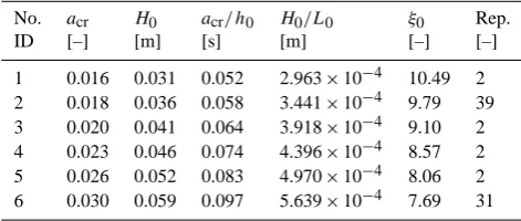
Table 1. List of sinusoidal waves used, values refer to measure-ments at the wavemaker, water depthh= is 0.31 m, periodT is 60 s, linear wave lengthL0becomes 104.63 m,ξ0surf similarity, no. of repetitions is given under “Rep”.
No. acr H0 acr/ h0 H0/L0 ξ0 Rep.
ID [–] [m] [s] [m] [–] [–]
1 0.016 0.031 0.052 2.963×10⁻⁴ 10.49 2
2 0.018 0.036 0.058 3.441×10⁻⁴ 9.79 39
3 0.020 0.041 0.064 3.918×10⁻⁴ 9.10 2
4 0.023 0.046 0.074 4.396×10⁻⁴ 8.57 2
5 0.026 0.052 0.083 4.970×10⁻⁴ 8.06 2
6 0.030 0.059 0.097 5.639×10⁻⁴ 7.69 31
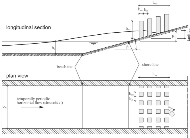
The problem of long waves which are climbing up a plane, sloping beach after propagating over a horizontal bottom is depicted in Fig. 1. Firstly, before the wave front reaches the shoreline, shoaling and refraction constitutes the main wave modification. At a specific water depth or for specific nonlin-earity wave breaking may occur. Yet, Madsen and Fuhrman (2008) pointed out that wave breaking is mostly dedicated to shorter waves riding on top of lower frequent tsunami waves. Then, during their run-up and subsequent draw-down, the approaching tsunami may interact with beachfront develop-ment represented in this study by MR eledevelop-ments positioned at different distances to each other and in different arrange-ments on the beach above the still water line. In order to re-peat this model situation, it is assumed that the first row of MR elements is always at the same distance to the still water line. One possible element combination as well as a longi-tudinal cross section are sketched schematically in Fig. 1, to demonstrate the model assumptions. Though the waves un-der consiun-deration are indeed longer than the slope applied for the experiments, the setting is illustrated in Fig. 1 with spa-tially shorter waves for the sake of clarity. For details of the applied waves the reader is referred to Table 1.
Additionally, two top-view movies depicting a sample lab-oratory experiment are provided as supplementary material that illustrate how a long wave principally reaches beach-front development modelled by a staggered, rotated MR el-ement configuration and then progresses through the urban agglomeration. Both wave run-up and subsequent draw-back are captured.
2 Theoretical framework
b
b
ch
mr bst
beach toe shore line
hmr
R
Lmr
tan
L
β
mr
temporally periodic horizontal flow (sinusoidal)
b
a h0
longitudinal section
plan view
Fig. 1. Schematic sketch of the problem set-up and the definition of the used variables,h0water depth,αangle of rotation of MR,βslope angle,Rwave run-up,bmrandhmrwidth and height of the macro-roughness elements,bstdistance between the macro-roughness elements. Spatial extent of the shown wave is not to scale. Experimentally investigated wave length significantly exceeds beach length (cf. Table 1).
the determination of key parameters that influence the pro-cess. Hence it is possible to limit experimental efforts to the most relevant parameters. In this study a variation of the surf similarity parameter in the aforementioned range is chosen.
2.1 Analytical wave run-up
Wave run-up was extensively studied in literature. Most com-monly, the work of Hunt (1959) is referenced who repro-cessed former published experimental studies, conducted ad-ditional experiments and analysed these aiming at design of sea walls and breakwaters. For breaking waves, the non-dimensional run-up becomes a function of beach slope, inci-dent wave height and wave steepness which reads
R H0
=ξ0=tanβ
H
0 L0
(−1/2)
for 0.1< ξ0<2.3, (1)
whereR/H0denotes the relative run-up normalized by the deep water wave heightH,ξ0is the surf similarity parame-ter. The angleβ denotes the beach slope. The non-breaking upper limit of wave run-up on a uniform slope is then given according to CEM US Army Corps (2002) reading
R H0
= √
2π
π
2β
1/4
. (2)
Equations (1) and (2) were derived on the basis of experi-mental research and thus the validity is limited to steep beach
slopes between 1/10 to vertical walls. Hence, additional for-mula have to be applied in the present cases where much milder slopes were investigated.
In the sequel, also solitary waves (Synolakis, 1987) or
N waves (Tadepalli and Synolakis, 1994) were addressed in connection with long-wave run-up. Often, the run-up formu-las reported in literature were derived empirically and for the special conditions used in this research with long-wave pe-riods and very mild beach slopes it is questionable if these approaches are valid to compare our experimental results with. However, recently Madsen and Schäffer (2010) pro-posed analytical solutions for the run-up and run-down based on the non-linear shallow water wave theory for various wave forms, where the duration and the wave height could be spec-ified separately in order to overcome the length scale de-ficiency of available long-wave models. This analytical ap-proach resulted in establishing run-up/run-down and veloc-ity formula for various waveforms such as isocelesNwaves, single waves and sinusoidal waves but with the important ex-ception that these waveforms did no longer exhibit a tie to wave height-to-depth ratio. The normalized run-up is sum-marized as a function of the surf similarity parameter de-rived, which reads (Madsen and Schäffer, 2010)
R a0
=χelevπ1/4
a
0 h0
−1/4
ξ0−1/2, (3)
h0 is offshore water depth. Surf similarity (ξ) is given by Eq. (4), which is based on the previously defined surf simi-larity Eq. (B5) but is recast by Madsen and Schäffer (2010) in terms of the effective durationof the wave. It reads
ξ= √
π
a
0 h0
−1/2 2h 0 gtanβ2
−1/2
, (4)
where tanβdescribes the beach slope. A theoretical breaking criterion is equally given by Eq. (5) (Madsen and Schäffer, 2010)
Rbreak a0
= 1
πξ
2. (5)
For the experiments presented in this study, the analytical run-up formula derived by Madsen and Schäffer (2010) is applied for the purpose of result comparison.
2.2 Definition of beachfront obstruction
In order to apply a measure for the beachfront obstruction a number of variables are introduced to express the influence of MR elements on the wave run-up. Geometrical definitions are sketched in Fig. 1. Most importantly, one has to define cross (ψcs) and long-shore rates of obstruction (ψls). Besides these horizontal obstruction rates, a component expressing the vertical obstruction of the flow cross section (ψmr) could be named similarly. Yet, vertical obstruction is only relevant when overtopping of MR elements is concerned which shall be excluded for the moment. The cross-shore obstruction ra-tio can be defined as
ψcs= Lmr nbmrˆ =
nbmrˆ +bst−bst
nbmrˆ =
n (bmr/cosϕ+bst)−bst nbmr/cosϕ
, (6)
where bˆmr=bmr/cosϕ denotes the width of the MR ele-ments according to their angle of rotation to the incident wave direction (cf. Fig. 4). The length of the obstructed beach in the direction of wave run-up is namedLmr, which can be defined as follows
Lmr=n (bmr+bst)−bst, (7)
withndenoting the number of MR element rows parallel to the still water line,bmrdefines the edge length of a single MR element andbstdefines the distance from one MR element to the next (i.e. street width). The cross-shore rate of obstruction depends on the ratio of the number of element rows times the width to the length of the macro-roughness area in on-shore direction. This geometrical ratio accounts for the obstruction exposed to the in-land propagating flow. The ratioψcs de-creases if the street width tends to zero,bst→0. The ratio grows if the number of MR rows is increased. The long-shore obstruction ratio is given by
ψls=
ˆ
bmr
ˆ
bmr+bst
= bmr/cosϕ
bmr/cosϕ+bst
, (8)
wherebˆ
mrequally expresses the effective width of the MR el-ements with respect to the approaching wave front. The long-shore rate of obstruction increases according to Eq. (8) when the ratio of the macro-roughness width to the sum of the street width plus the macro-roughness element width tends to unity. A long-shore rate of obstruction of unity is equiva-lent to a complete obstruction of the beach and results in full reflection of the wave and the run-up tongue. The above def-initions are used to evaluate the change in long-wave run-up with respect to the incoming waves.
3 Experimental set-up
Building on the theoretical framework described above, the experimental set-up and the related experimental programme is outlined in the following. Results of dimensional analy-sis are utilized to decide which variables have to be var-ied. Details of the varied variables are reported in Sect. 3.2. Froude similitude is chosen to downscale prototype condi-tions since from dimensional analysis (cf. Appendix B) it can be ruled out that viscosity and surface tension may – under the constraint of too tiny length or timescales – falsify run-up measurements significantly. The wave flume, its compo-nents to generate long waves as they are possibly generated by tsunamigenic sub-sea earthquakes as well as wave genera-tion methodology have recently been described by Goseberg (2011, 2012) and Goseberg et al. (2013); readers are referred to those publications for detailed information whereas a brief outline is presented in Sect. 3.1.
3.1 Wave flume
The experiments were carried out in the closed-circuit wave flume (race-track type) at the Franzius-Institute for Hy-draulic, Waterways and Coastal Engineering. A schematic drawing of the 56.94 m long flume illustrates the principal design of the facility (Fig. 2). The clear width of the flume amounts to 1.00 m. The flume is made of two parallel and 19.00 m long straights whose ends are connected by two semicircles of 6.87 m diameter. While one of the straights ac-commodates the run-up region, the other integrates a pump station that allows for the acceleration and deceleration of the water body. The water depth is kept constant at 0.31 m during all the reported experiments.
Fig. 2. Schematic drawing of the closed-circuit flume and its equipments, (a) pump station, (b) propagation section, (c) reservoir section, (d) sloping beach, (e) water storage basin (units in metre).
3.2 Test programme
In this study single sinusoidal waves with a fixed period
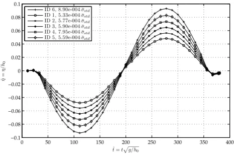
T =60 s were used to study the onshore interaction of long waves and beachfront development. In literature, many stud-ies exist that apply solitary waves when tsunami evolution in the vicinity of the shoreline is investigated (e.g. Synolakis, 1987). Few studies yet are based on cnoidal waves (Mo-ronkeji, 2007) while a variety of publications apply dam-break induced bores to study forces on free-standing struc-tures on the beach (Ramsden, 1996). Following the argumen-tation of Madsen et al. (2008) it recently became question-able if solitons are well suitquestion-able to serve as a model for near-shore tsunami. A main argument from the authors was that solitons lack in terms of geophysical time- and length-scales that are typical of tsunami. This argument was recently un-derlined by offshore GPS and bottom pressure measurements at the Japanese coast originating from the 2010 Chilean earthquake detecting wave periods much longer than those replicable from the solitary wave assumption (Kawai et al., 2012). Additionally, with respect to the overarching goal to study the influence of beachfront development to the long-wave run-up, the total duration of the interaction becomes important, which is comparatively short for commonly used solitary waves or Gaussian humps. Hence, it was deliberately chosen to step back to the most simple wave form possible in the laboratory. With respect to the length and timescales cho-sen, a period ofT =60 s was applied in this study leading to prototype condition periods ofT =600 s which is well in the range of measured realistic tsunami periods. Furthermore due to time constraints only leading depression waves were tested so far. Figure 3 presents the investigated waves with amplitude variations. Those applied single period sinusoidal waves consist of a leading wave trough followed by a wave crest. Prior and after these single sinusoidal wave periods sur-face elevation is kept constant at zero. Standard deviation is
0 50 100 150 200 250 300 350 400
−0.1 −0.08 −0.06 −0.04 −0.02 0 0.02 0.04 0.06 0.08 0.1
ˆ t=tp
g/h0
ˆ
η
=
η/
h0
ID 6, 8.90e-004 ¯σstd ID 1, 5.33e-004 ¯σstd ID 2, 5.77e-004 ¯σstd ID 3, 5.90e-004 ¯σstd ID 4, 7.95e-004 ¯σstd ID 5, 5.59e-004 ¯σstd
Fig. 3. Averaged non-dimensional surface elevation history for the six utilized waves, the markers denote the different waves heights,
¯
σstd is the averaged standard deviation calculated from the entire number of experiments in each group.
additionally given in order to show quality of the generated waves and their repeatability. Due to a lack of instrumenta-tion, no particle velocities under the wave trough and crest were measured continuously, though this depicts an interest-ing future research objective for the applied innovative wave generation method. Particle velocities were only measured a few times with a mobile current metre. Those resulting hor-izontal particle velocities yielded values in the range of the regime of the linear shallow-water wave theory; yet, further research is needed and will be published at a latter stage.
b
/sin(45°)
mr
bmr
bst
staggered, non-rotated
bst bmr
bst
bst
bmr
staggered, rotated
Fig. 4. Symmetry requirements for the configuration of the MR el-ements for a staggered, non-rotated configuration (left) and a stag-gered rotated configuration (right), drawing not to scale, demonstra-tion of the axis of symmetry at the flume wall, which always cuts an MR element in the half.
The MR elements were manufactured as solid, cubic blocks with an edge length of 0.10 m manufactured with a standard concrete mixture. As form work a standard cube mold was utilized to pour in the concrete. A total number of 100 complete cubes and 20 half cubes were manufactured. Figure 5 depicts an example configuration of the MR ele-ments in the flume. One notices some minor imperfections stemming from the production process of the MR elements (blowholes, dents) but in summary the quality of the con-crete cubes and their surfaces is regarded to be satisfactory for the experiments. Table 2 further outlines the number of experiments and the applied wave conditions during the ex-periments. With respect to the MR configurations different total numbers of experimental runs were possible.
The varied variables leading to the total number of ex-perimental runs are the distance between the elements (bst), the number of MR element rows (n), the angle of the ele-ments with respect to the incident wave direction (ϕ) and the choice of an offset between the element rows. In case of the aligned configuration (“al” in Table 2), four street widths were realized in the flume which are 2.5 cm, 4.2 cm, 6.6 cm and 10.0 cm, whereas for the staggered configuration (“st” in Table 2) only three street widths were used (2.5 cm, 5.9 cm, 10.9 cm). This is because the flume width is limited to 1.0 m. Two element angles ϕ∈(0◦,45◦) are further conceivable. Additionally, three different numbers of macro-roughness el-ement rows were tested in order to investigate the influence of the obstructed long-shore length,n∈(1,5,10). A prereq-uisite for the experiments was the strict compliance of two-dimensionality and thus symmetry. In preliminary experi-ments it was found that the application of whole-numbered distances between the MR elements led to large deviations of the maximum measured run-up compared to cases where symmetry conditions directly at the flume walls were meet. Figure 4 depicts two examples of MR configuration in the flume were correct application of symmetry was given.
Table 2. Number of conducted experiments classified according to the utilized wave properties listed in Table 1 and to the MR combi-nations0, “al” aligned, “st”’ staggered.
ID w/o MR al al st st 6
ϕ=0◦ ϕ=45◦ ϕ=0◦ ϕ=45◦
0=1 0=2 0=3 0=4
1 2 12 9 8 6 37
2 39 12 9 8 6 74
3 2 12 9 8 6 37
4 2 12 9 8 6 37
5 2 12 9 8 6 37
6 31 13 10 8 6 68
6 78 73 55 48 36 290
In both cases it was required to correctly close any dis-tances left between the half MR elements and the flume walls in order to circumvent any flow through these gaps. Addi-tional photographs of these wall and symmetry treatments are shown in Fig. 5.
3.3 Measurements and instrumentation
In order to evaluate run-up reduction due to the interaction of the incoming waves with the beachfront development, a large set of parameters was recorded. Besides the measurement of surface elevations along the horizontal bottom, water depths were collected on the beach slope. The maximum run-up was captured with a drift-line approach. Additionally, flow veloc-ities were recoded at selected positions along the propagation path. A comprehensive sketch of positions of sensors is given in Fig. 6.
Fig. 5. Photographs of the MR element implementation. Left: Example of a staggered MR element configuration, Right: Half cubes used at the flume walls.
inspection window
shore
line
X Z UDS_1
PRS_7 PRS_6
PRS_5
PRS_4 PRS_3 PRS_2 PRS_1
RWG_3 RWG_2
RWG_1
beach
toe
flume curve
shore
line beach
toe
X
Y PRS_1
RWG_1 RWG_2 RWG_3 PRS_2
PRS_3 PRS_4
PRS_5 PRS_6 PRS_7 UDS_1
inspection window
inspection window
flume
curv
e
0.50
0.50
0.46
0.54
1.42 0.24 0.40 1.00 1.00 1.00 2.05 2.87 2.00 2.00 0.39 0.92
Fig. 6. Layout drawing of the laboratory instrumentation with used pressure sensors and wave gauges for the experimental set-up, abbrevia-tions denote the following devices: PRS – pressure sensor, RWG – resistance wave gauge, UDS – ultrasonic distance sensor; for more than one device consecutive numbers are given, not to scale (units in metre), note that some sensors are not analysed in this paper.
the PVC board surface rectangularly pointing to the beach inclination.
The detection of the maximum wave run-up is of key im-portance in this study. Besides visual detection, beach par-allel capacitive type wave gauges (Oumeraci et al., 2001) or camera-based techniques are feasible. Alternatively to these methods, in this study a drift-line-based approach is chosen to detect the maximum run-up of the waves. The basic idea resembles drift lines along natural beaches where deposited debris is one potential demarcation of the highest run-up of the incoming sea condition. Analogously, in this experiment
Rmax Rmin
Rmean
Fig. 7. Maximum wave run-up detection in the laboratory defined as the mean (Rmean) of the lowest (Rmin) and the highest maximum run-up (Rmax).
energy dissipation in the boundary layer of the flume walls. The reported wave run-up, which is referred to in the fol-lowing, is therefore defined as the mean of the lowest and the highest maximum run-up measured in each experimental run. Figure 7 exemplifies how the lowestRminand the high-est maximum run-upRmaxwere defined. In order to circum-vent influences from wall effects, areas as close as 0.05 m to the flume walls were excluded from the run-up determi-nation. After determination of minimal and maximal run-up, average values were recorded.
3.4 Experimental procedure and data processing
A typical experimental procedure encompasses the wave generation described in Sect. 3.1 along with the run-up mea-surements, the wave height and water depth measurements at various positions as well as the velocity measurements de-scribed in Sect. 3.3. After a long wave was generated it prop-agated along the flume and climbed up the sloping beach un-til its maximum run-up elevation was reached. Thereafter the particle velocity turned negative and the run-down phase fol-lowed.
Data processing aimed at converting, filtering, smoothing and decimating recorded signals. For some reasons an inter-nal sampling rate of 1.0 kHz was applied; thus decimation was accomplished by extracting every fiftieth data point from the signal subsequently after filtering and smoothing took place. Data were stored in a digital experimental notebook where in addition to the measured data, processed variables such as the configuration tag0, the vertical run-upRv,min, Rv,max, the long- and cross-shore obstruction ratioψls,ψcs, the wave periodT, crest acr and troughatr amplitudes and wavelength L0 at the wavemaker, the wave number k, the frequencyand the surf similarity parameter ξ0. Filtering with good results was obtained on the basis of the empirical mode decomposition (EMD) technique (Huang et al., 1998).
0.04 0.05 0.06 0.07 0.08 0.09 0.1 0.11
3 3.1 3.2 3.3 3.4 3.5 3.6 3.7 3.8 3.9 4
acr/h0
Rm
e
a
n
/
acr
0.50 maxacr 0.60 maxacr 0.70 maxacr 0.80 maxacr 0.90 maxacr 1.00 maxacr Polynomial fitting,m= 1
Fig. 8. Maximum relative run-up as a function of the nonlinearity () of the waves depicted by the markers, a linear polynomial fit de-notes the increase in maximum run-up with increasing nonlinearity.
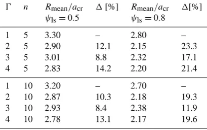
Table 3. Summary of normalized run-up and relative differences with regard to configuration 0=1 for MR element rows with n= 5; 10, listed values base on the polynomial fitting curves.
0 n Rmean/acr 1[%] Rmean/acr 1[%]
ψls=0.5 ψls=0.8
1 5 3.30 – 2.80 –
2 5 2.90 12.1 2.15 23.3
3 5 3.01 8.8 2.32 17.1
4 5 2.83 14.2 2.20 21.4
1 10 3.20 – 2.70 –
2 10 2.87 10.3 2.18 19.3
3 10 2.93 8.4 2.38 11.9
4 10 2.78 13.1 2.17 19.6
4 Results
The wave run-up of single, sinusoidal waves was investigated by means of scale experiments. Basically wave height was varied and surf similarities between ξ =7.69–10.49 were achieved. Firstly 78 experiments were conducted to anal-yse the run-up on a plain 1 in 40 sloping beach without any surface-piercing MR objects. These results are addressed in Sect. 4.1. Subsequently, experiments were conducted that fo-cus on the long-wave run-up reduction due to MR elements which were arranged in four different patterns on the shore, details are listed in Table 2. Resulting reduced run-up is de-scribed in Sect. 4.2. Additionally, in Sect. 4.4 it is qualita-tively presented how the surface elevation evolves with and without MR elements on the shore in a longitudinal direction.
4.1 Undisturbed run-up
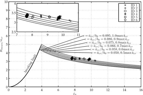
0 2 4 6 8 10 12 14 16 0 1 2 3 4 5 6 7 8 ξ0 Rm e a n /
acr
ǫ= ¯acr/h0= 0.050, 0.5max ¯acr ǫ= ¯acr/h0= 0.058, 0.6max ¯acr ǫ= ¯acr/h0= 0.066, 0.7max ¯acr ǫ= ¯acr/h0= 0.075, 0.8max ¯acr ǫ= ¯acr/h0= 0.086, 0.9max ¯acr ǫ= ¯acr/h0= 0.095, 1.0max ¯acr
brea kin gli mit ID 5 ID 6
7 8 9 10 11
2.5 3
Fig. 9. Maximum relative run-up as a function of the surf similarity parameter (ξ0) depicted by the markers and according to the wave conditions applied, the theoretical breaking limit given by Eq. 5 and the theoretical run-up functions given by Eq. 3 (Madsen and Schäf-fer, 2010) based on the non-linearity (). The inset zooms to the experimental data.
In this research basically the wave nonlinearity 2a0/ h0was varied leading to the variation of surf similarity as men-tioned before. Figure 8 depicts the maximum relative run-upRmean/acras a function of the nonlinearity=acr/ h0of the investigated waves. Here, the maximum relative run-up is defined as the average of the measured run-up outlined in Sect. 3.3. The general trend of the measured data set is expressed by the polynomial fit of the degreen=1 which basically reduces to a linear function.
Since the overall aim was to investigate wave run-up re-duction due to MR elements onshore, no further variations of the wave periodT and the beach slope tan(β)were accom-plished in this research. In tendency, it becomes clear that an increasing nonlinearity results in increasing relative run-up. Yet, only non-breaking conditions were tested. It is also obvi-ous that the relative run-up related to the positive crest ampli-tude is remarkably high. It ranges betweenRmean/acr=3.1– 3.4. In order to check whether our data sets are consistent with existing research, Fig. 9 presents the maximum relative wave run-up in the framework of the surf similarity param-eter (cf. Eq. 3 and Madsen and Schäffer, 2010). The max-imum relative run-up, which is normalized by the positive amplitude at the wavemaker, decreases with an increasing surf similarity parameter ξ0. The increase in non-linearity, which can be expressed as the ratio of the applied wave am-plitude of the crest acr/ h0, reduces the surf similarity of the applied wave condition at the beach under investigation. Higher non-linearity of the wave also indicates higher energy content. This finding underlines the statement of Madsen and Fuhrman (2008) after which critical flow depth and flow ve-locities occur for surf similarity in the order ofξ0=3–6 and in turn require relatively mild beach slopes.
0 0.1 0.2 0.3 0.4 0.5 0.6 0.7 0.8 0.9 1
1 1.5 2 2.5 3 ψls Rm e a n /
acr ID 1
ID 2 ID 3 ID 4 ID 5 ID 6
No macro roughness Polynomial fitting, m=2 Extrapolation area
0 0.1 0.2 0.3 0.4 0.5 0.6 0.7 0.8 0.9 1
1 1.5 2 2.5 3 3.5 4 ψls Rm e a n /
acr
Γ = 1, n= 5, ϕ= 0◦,arrangement: aligned
p(x) =−13.79x2+ 22.68x1+−13.52
ID 1 ID 2 ID 3 ID 4 ID 5 ID 6
No macro roughness Polynomial fitting, m=2 Extrapolation area
0 0.1 0.2 0.3 0.4 0.5 0.6 0.7 0.8 0.9 1
1 1.5 2 2.5 3 3.5 4 ψls Rm e a n /
acr
Γ = 1, n= 10, ϕ= 0◦,arrangement: aligned
p(x) =−8.44x2+ 11.80x1+−5.90
ID 1 ID 2 ID 3 ID 4 ID 5 ID 6
No macro roughness Polynomial fitting, m=2 Extrapolation area
Fig. 10. The relative wave run-up (Rmean) as a function of the long-shore obstruction ratio (ψcs),0=1. The experimental data are fit-ted to a polynomial of degreem=2 and the equations are given according to the investigated number of MR rowsn=1,5,10.
The resulting measurements depicted by the point clouds are in good agreement with the analytical framework. Yet, it is apparent that the results do not perfectly fit the expected analytical behaviour even though the results already indi-cate that the theory and the functional relation of the non-dimensional terms are well established. The analytical ap-proach fully neglects the influence of roughness and even though the experiments aim at eliminating roughness influ-ences to the greatest extent, energy losses due to roughness influence are still existent. From the degree of agreement be-tween the experimental data and the analytical approach it can thus be reasoned that the experimental set-up is in princi-pal suitable to reproduce long-wave motion in scaled models and in the following it shall be demonstrated how MR ele-ments contribute to reduced long-wave run-up quantitatively.
4.2 Run-up reduction
the Appendix. According to Table 2 four MR configurations were tested and results are presented in this section subse-quently. Additional plots are presented in the Annex. Firstly, the relative run-up of long waves normalized by the posi-tive wave amplitude at the wavemaker is shown in Fig. 10 as a function of the long-shore obstruction ratio (Eq. 8) where long-shore obstruction ratio of unity denotes full obstruction of the beach section. Equally, a zero long-shore obstruction ratio indicates that no obstacles are present on the beach and those cases are represented in Fig. 10 by the star symbol. As shown, not much difference in relative run-up is found be-tweenψls=0.5 and the limiting case ofψls=0.0
The MR configuration0=1 comprises MR elements in aligned arrangement with non-rotated elements. The result-ing run-up reduction can generally be described by a down-ward opening parabolic function. Note that two of the exper-iments were excluded from the analysis because measured run-up appeared to be non-physical. Four different long-shore obstruction ratios were tested. Long-wave run-up di-minishes with increasingψls. It appears that the influence of the incident wave amplitude indicated by the marker symbols tends to increase with an increasing long-shore obstruction ratio. Higher incident wave amplitudes result in higher water levels in the vicinity of the macro-roughness area. A reason for this finding could be that higher velocities in between the MR openings result in higher energy exchange between the predominant inland-directed flow and the calmed areas in the back of MR elements; thus leading to increasing energy dis-sipation. This observation agrees with the findings of Goto and Shuto (1983) who investigated the effects of wooden pil-lars exposed to a steady flow and similarly reported momen-tum exchange between the main flow and eddies in the back of their obstacles. Figure 10 also indicates that the number of MR element rows (n) has a much smaller influence on the maximum run-up reductions. For values ofψls=0.8 only marginal differences exist between the relative run-up reduc-tion (Rmean/acr). Yet, it appears that the scatter of the mea-sured run-up slightly increases to some extent, which could be attributed to an increase in turbulence when the flow in-teracts with a higher number of MR element rows.
According to the tabulated results presented in Table 3 the highest run-up reduction is achieved by MR configura-tion 0=2 which depicts the aligned, rotated case (cf. Ta-ble 2). This configuration leads to additional run-up reduc-tion of 21.3 % forψls=0.8 whenn=5 MR element rows are tested. This reduction slightly decreases for the case with
n=10 MR element rows which at first contradicts the state-ment that energy reduction increases with increasing number of MR element rows. Although here, this opposed trend is rather related to the scatter of data that leads to variations in the polynomial fitting curves applied for the summary ta-ble. The influence of the MR angle is further described and discussed in Sect. 4.3.
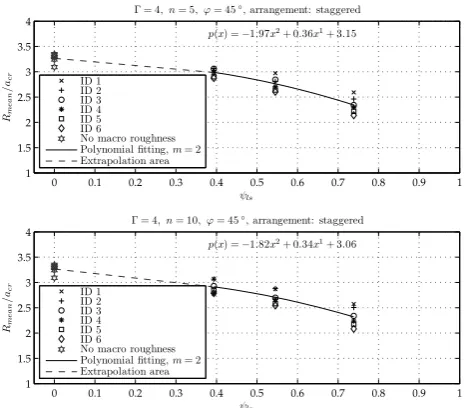
0 0.1 0.2 0.3 0.4 0.5 0.6 0.7 0.8 0.9 1
1 1.5 2 2.5 3 3.5 4
ψls Rm
e
a
n
/
acr
Γ = 4, n= 5, ϕ= 45◦,arrangement: staggered
p(x) =−1.97x2+ 0.36x1+ 3.15
ID 1 ID 2 ID 3 ID 4 ID 5 ID 6
No macro roughness
Polynomial fitting,m= 2
Extrapolation area
0 0.1 0.2 0.3 0.4 0.5 0.6 0.7 0.8 0.9 1
1 1.5 2 2.5 3 3.5 4
ψls Rm
e
a
n
/
acr
Γ = 4, n= 10, ϕ= 45◦,arrangement: staggered
p(x) =−1.82x2+ 0.34x1+ 3.06
ID 1 ID 2 ID 3 ID 4 ID 5 ID 6
No macro roughness
Polynomial fitting,m= 2
Extrapolation area
Fig. 11. The relative wave run-up (Rmean) as a function of the long-shore obstruction ratio (ψls),0=4. The experimental data are fit-ted to a polynomial of degreem=2 and the equations are given according to the investigated number of MR rowsn=5,10.
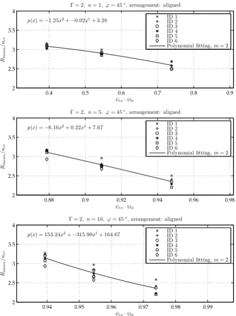
In order to incorporate the non-dimensional variable cross-shore obstruction ratio (ψcs) it is convenient to define an ad-ditional non-dimensional variable that accounts for the entire horizontal obstruction ratio. It may read
ψ2-D=ψcsψls. (9)
Equation (9) relates the long- and the cross-shore obstruc-tion ratio. While the long-shore obstrucobstruc-tion ratio resides be-tween zero and unity, the cross-shore obstruction ratio, by definition, reaches unity if only one macro-roughness row is considered and decreases with a growing number of macro-roughness element rows. For one MR element row the prod-uct ofψcsandψlsreduces to the long-shore obstruction ratio (ψls), whereas it grows with an increasing number of ele-ment rows. It has to be noted that the 2-D obstruction ra-tio is based on the assumpra-tion that the street widths in the cross- and long-shore direction are equal. As an example, Fig. 12 presents the normalized run-up as a function of the two-dimensional obstruction ratioψ2-Daccording to Eq. (9) for the case of0=2 with rotated elements in an aligned ar-rangement.
0.4 0.5 0.6 0.7 0.8 0.9 2
2.5 3
ψcs·ψls Rm
e
a
n
/
acr
ID 4 ID 5 ID 6
Polynomial fitting,m= 2
0.88 0.9 0.92 0.94 0.96 0.98
2 2.5 3 3.5 4
ψcs·ψls Rm
e
a
n
/
acr
Γ = 2, n= 5, ϕ= 45◦,arrangement: aligned
p(x) =−6.16x2+ 0.22x1+ 7.67
ID 1 ID 2 ID 3 ID 4 ID 5 ID 6
Polynomial fitting,m= 2
0.94 0.95 0.96 0.97 0.98 0.99
2 2.5 3 3.5 4
ψcs·ψls Rm
e
a
n
/
acr
Γ = 2, n= 10, ϕ= 45◦,arrangement: aligned
p(x) = 153.24x2+−315.90x1+ 164.67 ID 1ID 2
ID 3 ID 4 ID 5 ID 6
Polynomial fitting,m= 2
Fig. 12. The relative wave run-up (Rmean) as a function of the cross-shore obstruction ratio (ψcs) times the long-shore obstruction ratio (ψls),0=2. The experimental data are fitted to a polynomial of de-greem=2 and the equations are given according to the investigated number of macro-roughness rowsn=1,5,10.
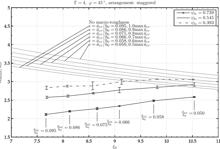
From an engineering perspective it is preferable to either yield empirical equations or derive nomograms which are suitable to predict the reduced run-up due to a given MR configuration in comparison with the undisturbed case. Be-sides the specific MR element configuration, it is the long-shore obstruction ratio that basically dominates the run-up reducing effect of the investigated MR elements as a func-tion of the cross-shore obstrucfunc-tion ratio, as outlined above. On that basis it is convenient to focus on the dominating long-shore obstruction ratio (ψls) to deduce conclusions from the experimental findings. Figures 13 and 14 illustrate the re-lation of the relative run-up (Rmean/acr) to the surf similar-ity parameter (ξ0) within the analytical framework of Mad-sen and Schäffer (2010) for the MR configurations0=2,4. Nomograms referring to the configurations0=1,3 are pre-sented in the annex for completeness. The reduced relative run-up according to the MR elements on the shore is ex-pressed by means of the long-shore obstruction ratio and is plotted as a error bar line where the line denotes the aver-aged run-up of the casesn=1, n=5 and n=10. The er-ror bars mark the standard deviation of the measured relative
tio slightly decreases with an increasing non-linearity of the applied waves, which is most likely contributed to greater momentum exchange within the MR element area. Six error bars for each long-shore obstruction ratio indicate those wave conditions tabulated in Table 1.
For both nomograms presented in Figs. 13 and 14, the re-duction of the relative run-up decreases slightly with decreas-ing surf similarity (ξ). The reduction of the relative run-up compared to undisturbed conditions is less significant for a long-shore obstruction ratio ofψls=0.393; yet, it appears that the maximum run-up tends to zero when the long-shore obstruction ratio is further increased. Standard deviation of measured relative run-up is rather small indicating that most of the experimental results are fairly repeatable. Secondly, it can be observed that the relative run-up again decreases with an increase in non-linearity, which is probably contributed to the growth in momentum exchange when waves of higher non-linearity interact with the MR elements. Higher turbu-lence production is assumed to affect the increase in run-up reduction.
4.3 Influence of the MR angle
In contrast to the aligned MR configurations, Fig. 11 depicts MR configuration0=4 where MR elements are arranged in a staggered manner and rotated by the angle ϕ=45◦. The functional dependency between normalized run-up and long-shore obstruction ratio is similar to the aligned, non-rotated configuration. A parabolic polynomial is also suitable to fit the measured data. The extrapolated region between
ψls=0.5 and 0.0 is indicated by a dashed line while the run-up results without consideration of obstacles on the beach are represented by some stars. Yet, the run-up reduction is higher than in the non-rotated cases. A summary of the re-sults and the comparison of investigated MR configurations is presented in Table 3.
In comparison with non-rotated MR configuration0=1 a substantial additional run-up reduction could be found for configuration0=4 (cf. Fig. 4, right panel). It appears that for cases withn=5 MR element rows in staggered, rotated configuration, the normalized run-up decreases by 4.2 % for
ψls=0.5 and by 21.4 % for ψls=0.8, while in case of n=10 MR element rows those reductions are 13.1 % for
ψls=0.5 and 19.6 % forψls=0.8, respectively. Addition-ally, some scatter is introduced into the data in the case of
7 7.5 8 8.5 9 9.5 10 10.5 11 1.5
2 2.5 3 3.5 4 4.5 5
ξ0
Rm
e
a
n
/
ac
r
¯
ac r
h0 = 0.050
¯
ac r
h0 = 0.058
¯
ac r
h0 = 0.066
¯
ac r
h0 = 0.075
¯
ac r
h0 = 0.086
¯
ac r
h0 = 0.095
Γ = 2, ϕ= 45◦,arrangement: aligned
ψls= 0.739
ψls= 0.545
ψls= 0.393
7 7.5 8 8.5 9 9.5 10 10.5 11
1.5 2 2.5 3 3.5 4 4.5 5
ǫ= ¯acr/h0= 0.050, 0.5max ¯acr
ǫ= ¯acr/h0= 0.058, 0.6max ¯acr
ǫ= ¯acr/h0= 0.066, 0.7max ¯acr
ǫ= ¯acr/h0= 0.075, 0.8max ¯acr
ǫ= ¯acr/h0= 0.086, 0.9max ¯acr
ǫ= ¯acr/h0= 0.095, 1.0max ¯acr No macro-roughness
Fig. 13. The relative wave run-up (Rmean/acr) as a function of the surf similarity parameter (ξ0),0=2. The experimental data are plotted according to the individual long-shore obstruction ratio. The error bars indicate the variation of the number of macro-roughness element rows. The grey parallel graphs indicate the relative run-up without the interaction with macro-roughness. The non-linearity of the applied waves is indicated as text which always refers to all error bars in the vertical above.
7 7.5 8 8.5 9 9.5 10 10.5 11
1.5 2 2.5 3 3.5 4 4.5 5
ξ0
Rm
e
a
n
/
ac
r
¯
ac r
h0 = 0.050
¯
ac r
h0 = 0.058
¯
ac r
h0 = 0.066
¯
ac r
h0 = 0.075
¯
ac r
h0 = 0.086
¯
ac r
h0 = 0.095
Γ = 4, ϕ= 45◦,arrangement: staggered
ψls= 0.739
ψls= 0.545
ψls= 0.393
7 7.5 8 8.5 9 9.5 10 10.5 11
1.5 2 2.5 3 3.5 4 4.5 5
ǫ= ¯acr/h0= 0.050, 0.5max ¯acr
ǫ= ¯acr/h0= 0.058, 0.6max ¯acr
ǫ= ¯acr/h0= 0.066, 0.7max ¯acr
ǫ= ¯acr/h0= 0.075, 0.8max ¯acr
ǫ= ¯acr/h0= 0.086, 0.9max ¯acr
ǫ= ¯acr/h0= 0.095, 1.0max ¯acr
No macro-roughness
−10 0 10 20 30 40 50 −0.2
−0.1 0 0.1 0.2 0.3
x/h0
ˆ
η
=
η/
h0
ˆ
t=tp
g/h0= 337.41
Beach profile 1/40
−10 0 10 20 30 40 50
−0.2 −0.1 0 0.1 0.2 0.3 0.4
x/h0
ˆ
η
=
η/
h0
ˆ
t=tp
g/h0= 348.66
Fig. 15. Comparison of the normalized surface elevation for a sinusoidal wave with=0.093 attˆ=337.41 andtˆ=348.66 with and without the presence of macro-roughness elements. The macro-roughness element configuration is specified by0=4,ϕ=45◦,bst=0.025 and n=5. Surface elevation and spatial coordinates are normalized by the invariant water depth (h0). The dash-dotted line depicts the macro-roughness element area.
−10 0 10 20 30 40 50
−0.2 −0.1 0 0.1 0.2 0.3 0.4
x/h0
ˆη
=
η/
h0
ˆ
t=tp
g/h0= 539.93
Normalized surface elevation,ǫ= 0.093
No macro-roughness
Γ = 4ϕ= 45bst= 0.025n= 5
Beach profile 1/40
−10 0 10 20 30 40 50
−0.2 −0.1 0 0.1 0.2 0.3 0.4
x/h0
ˆη
=
η/
h0
ˆ
t=tp
g/h0= 551.18
As listed in Table 3, cases0=2 (aligned,ϕ=45◦) and 4
(staggered,ϕ=45◦) always depict higher run-up reductions
compared with the reference case0=1. In our opinion, this substantiates the conclusion that the influence of block angle is stronger than the influence of aligned or staggered arrange-ment. This result holds true for either 5 or 10 rows of MR elements (cf. Sect. 5).
4.4 Longitudinal evolution of surface elevation
Finally, the longitudinal evolution of the free surface ele-vation of the undisturbed long-wave run-up is compared to the MR configuration 0=4, a staggered and rotated con-figuration, with ψls=0.739 and n=5 MR element rows. Here, the qualitative influence of MR elements configura-tion to the spatial distribuconfigura-tion of the water level at dis-tinct time steps should be assessed. Out of the sequence of available time steps of the wave evolution along the beach wedge, Fig. 15 depicts the situation during wave run-up while Fig. 16 focuses on the draw-down phase. Time is given non-dimensionally with reference to the beginning of the wave generation at the wavemaker; thus, non-dimensional timetˆ=t√g/ h0relates to the total time for the wave needed to propagate along the horizontal bottom section and climb-ing up the 1 in 40 slopclimb-ing beach. Both figures illustrate the development of the surface elevation profile along the beach wedge. The normalized surface elevationηˆ=η/ h0is given as a function of the non-dimensional horizontal coordinate
ˆ
x=x/ h0. The position and the height of the obstacle area is given by the dash-dotted grey lines while the beach surface is presented by the full grey line. A wave with a non-linearity of=0.093 is used. Generally, three qualitative phases can be determined during the evolution of the wave. First of all the initial draw-back of the water, which is due to the leading depression wave character, characterizes the wave evolution. In this phase no significant differences can be found for the cases with and without MR elements. In a second phase when the water surface elevation is rising on the beach, in tendency higher water levels are determined for the obstructed case. Thirdly, during the draw-down of the long wave the situation inverts and the surface profile is lower for the case with MR elements present. The flow of water which is in-between and behind the MR area is retarded significantly (Fig. 16).
An interesting feature is demonstrated in Fig. 15. The ap-proaching wave tongue collides with the first MR element row and a shock wave is formed which propagates seawards. This flow feature is observed for all investigated long-shore obstruction ratios and for all MR configurations. The height of the shock wave qualitatively depends on the long-shore obstruction ratio, though this dependency has not been in-vestigated in detail in this research. The front of the initi-ated reflection wave is comparable with a monoclinal rising wave which though rapidly varies during its seaward propa-gation. In the presented case the surface gradient of the pos-itive surge, whose front is initially steep, decreases rapidly
and it flattens out noticeably (lower panel of Fig. 15). The situation inverts as soon as the long wave starts the draw-down process (Fig. 16). In the vicinity of the MR elements the undisturbed case faces higher water levels than in the case with MR elements. This is a direct result of the effect of the MR elements causing decreasing maximum wave run-up, since obstacles are causing partial reflections of the shore-ward transported wave energy. Finally, an additional feature appears within the MR element area. There, the water levels are higher with MR elements compared to the undisturbed case. This is due to the fact that the volume of water which at this time is situated in-between and behind the obstacles is retarded significantly and is only displaced during the draw-down phase with a notable time lag. In the case of MR it is apparent that the negative, seaward directed surface gra-dient in the vicinity of the obstacles is considerably higher than that without obstacles. In consequence, the flow veloc-ities are qualitatively increased compared to the undisturbed run-up.
5 Discussion
cordance with the long-wave theory and that, more impor-tantly, transverse velocity components inside the flume bend were marginal, so that no direct influence on the wave prop-agation is expected.
The basic flow features which were observed in the course of the run-up and draw-down phase of the wave climbing up the beach and interacting with the MR elements consist of acceleration and deceleration due to sudden narrowing and widening in between the MR element area. This pro-cess increases with reduction of long-shore obstruction ra-tio and with increasing non-linearity of the incident waves. These features directly influence the maximum run-up that was under investigation. These findings are in close agree-ment with previous findings for steady-state flows. For exam-ple, Soares-Frazão et al. (2008) qualitatively found the same flow pattern (sudden narrowing, widening and deceleration) in the case of a flood wave impinging an urban settlement of houses which are arranged in an aligned and staggered con-figuration. Similar findings were reported by Goto and Shuto (1983) and Soares-Frazão and Zech (2008).
Besides the fundamental flow features that were deter-mined, four different MR element configurations were tested with varying number of obstacle rows. A summary of abso-lute run-up and differences between those variations is pre-sented in Table 3. It appears that absolute run-up reduction for a given obstruction ratio depends on the kind of MR el-ement arrangel-ement (i.e. aligned or staggered). Aligned and staggered arrangements with identical angle of rotation yield differences of 8.4 to 8.8 % for 5 MR rows and 11.9 to 17.1 % for 10 MR rows. Yet, especially in case of the aligned con-figuration (0=1,2) the angle of rotation seems to have a greater contribution to the overall run-up reduction compared with the staggered configuration (0=3,4) where difference are less dominant. This effect is clearly seen with the increas-ing number of MR element rows. An increasincreas-ing effect of MR element rotation angle to the overall run-up reduction is also observed with increasing obstruction ratio which can be sub-stantiated by differences for configuration0=1,2 between
ψls=0.5,0.8. Differences in this case are almost doubled from 12.1 % to 23.3 %. A likely explanation of this fact is that an angle ofϕ=45◦results in much greater local momentum deflection at the MR elements than in non-rotated cases. The momentum deflection in turn leads to greater turbulence gen-eration in the zone where two opposing currents are collid-ing with each other and therefore a larger amount of energy is dissipated. Due to the greater energy dissipation, less en-ergy is maintained in the run-up tongue resulting in smaller overall run-up values. Hence from the results obtained by an comparison of effects due to angle of rotation and due to MR element configuration it is apparent that the angle of rotation stronger influences the overall run-up reduction than the dis-tinction of aligned or staggered configuration.
overall run-up of the researched waves for a 1 in 40 sloping beach. Contrary to prototype conditions, beachfront devel-opment was idealized by concrete cubic blocks which were arranged in a regular pattern. This approach significantly differs from prototype development in terms of structuring, where houses and infrastructure is mostly randomly dis-tributed. Nevertheless, the roughness effect to an incoming flow which is either exposed to a randomly build or a struc-tured development is maintained by defining cross- and long-shore obstruction ratios. This approach is based, of course, on the assumption that roughness effects considered over a larger onshore area cancel out local variability in MR ele-ment distribution. In order to compare the obtained results with a realistic prototype situation it is thus under this as-sumptions possible to check for the given obstruction ratios of an area under research. With those obtained values one might consider the nomograms for estimating possible run-up reduction; this method offers a rough estimation at least for beach slopes within the investigated range. Practically, the presented results could be applied to a given sample set-ting in the following steps;
– Determination of natural shelf or beach slope and
check of applicability to the presented results obtained from 1 in 40 beach slope experiments.
– Determination of cross- and long-shore obstruction
ra-tios through evaluation of Eqs. (6) and (8) (defini-tion of horizontal obstruc(defini-tion ratios) along some cho-sen transects parallel and orthogonal to the shoreline – Classification of the given beachfront development.
– Selection of most applicable arrangement of the
build-ing settbuild-ing with respect to arrangements0=1–4.
– Choice or review of wave parameters of a potential
tsunami at the particular location, e.g. wave height, du-ration or period and water depths in order to calculate a corresponding surf similarity parameter.
– Utilization of the associated nomogram (determined
surf similarity parameter and parameters of the classi-fied beachfront development) by reading off the undis-turbed tsunami. run-up as well as the run-up reduction predicted by the experimental results
Besides analysing the overall run-up reduction due to the presence of MR elements Figs. 15 and 16 depict some char-acteristic stages of the wave run-up and subsequent draw-down process in the vicinity of the first MR row. Note that the presented surface elevations show snapshots of the sur-face elevation. The overall (total) run-up could not be de-termined from the figures presented above. Compared with non-obstructed conditions, a shock wave is generally gen-erated at the first row of obstacles which starts propagating back offshore as soon as the wave tip reaches the MR ele-ments. This shock wave is considered to reflect some of the incoming wave energy though it has to be further researched quantitatively what contribution the beachfront development has to the overall reflection coefficients. In addition, the wave is retarded in a later stage of the run-up process and a volume of water is held back, since it is supposed to flow back to the sea through the opening between the MR elements in the first row. This is of great importance with respect to prototype conditions since it confirms the common belief that receding waters draw back slower in the vicinity of build environment than in regions where open land is found at the coastline.
6 Conclusions and outlook
The experiments reported herein address the problem of de-termining the reduction of maximum tsunami run-up on a 1 in 40 plane beach when the run-up process is disturbed by beachfront development in close proximity of the shoreline. The resistance of urban structures on the beach is modelled by means of MR elements made of cubic concrete blocks. The experimentally determined relative run-up of single si-nusoidal waves on the plane beach without MR elements agrees well with an analytical approach by Madsen and Schäffer (2010). For the first time this theoretical approach is successfully validated by experimental means. The rela-tive run-up of the waves under consideration is significantly influenced by the presence of MR elements onshore. As a re-sult, nomograms are presented to facilitate the determination of the relative run-up reduction for four different MR element configurations, various long- and cross-shore obstruction ra-tios and a range of wave non-linearities. Simple yet idealized predictions of the reduction of long waves due to MR ele-ment configurations are therewith made possible. The exper-imental data sets of long-wave run-up are also capable to be utilized for the calibration and validation of numerical mod-els.
It belongs to the character of laboratory idealizations that some aspects of the prototype process are still neglected. Among these aspects are influences stemming from the col-lapse of buildings, the transport of sediment and debris, the volumetric disequilibrium between solid blocks (in the present model) and common hollow buildings (in prototype), three-dimensional influences of river estuaries or heteroge-neous existing developments, different building orientations
and dimensions, the overflow of developments and spatially or temporally varying surface gradients. Moreover, the pre-sented material is believed to owe the potential to facili-tate future modelling approaches of beachfront development, though it is beyond the intention of this paper. The above mentioned aspects remain untreated and further laboratory work is needed to elucidate those additions to the interaction process of long waves and beachfront development.
Appendix A
Additional nomograms
Some more nomograms are provided in this section that add information about the remaining MR configurations0=1,3 for the sake of completeness.
Appendix B
Dimensional analysis and laboratory effects
B1 Dimensional analysis
Dimensional analysis was often utilized in the past to op-timise experimental research. It is an engineering tool that allows to express and describe physical processes by means of dimensionless terms after the dependent variables for the process have been deduced and delineated (Yalin, 1971). By means of the theorem of Buckingham it becomes possible to reduce an equation of the formf (x1, x2, . . . , xn)=0
con-tainingnphysical variablesxwith a dimension matrix of or-derrinto an equation of the formF (51, 52, . . . , 5n−r)=0
by recasting into dimensionless 5 terms. The dimension-less variables 5 are composed of power products of the former dimensional variables x. Undisturbed wave run-up was investigated by various authors (i.e. Hunt, 1959). Di-mensional analysis for this problem was addressed in de-tail by Müller (1995) who derived dimensional analysis for the problem of impulsive wave propagation and run-up in alpine lakes induced by rock fall. Limiting the problem to two-dimensionality, neglecting model, scale as well as fric-tional effects, relative run-up might be related to the follow-ing dimensional variables:
f
g, %, ν, ς
| {z }
universal properties
, a, T , β, c
| {z }
plain wave run-up
, bmr, bst, n, ϕ, 0
| {z }
MR related
=0, (B1)
wheregis gravitational acceleration,%is density of the fluid,
7 7.5 8 8.5 9 9.5 10 10.5 11 1.5
2 2.5 3 3.5 4 4.5
ξ0
Rm
e
a
n
/
ac
r
¯
ac r
h0 = 0.050
¯
ac r
h0 = 0.058
¯
ac r
h0 = 0.066
¯
ac r
h0 = 0.075
¯
ac r
h0 = 0.086
¯
ac r
h0 = 0.095
ψls= 0.704
ψls= 0.602
ψls= 0.500
7 7.5 8 8.5 9 9.5 10 10.5 11
1.5 2 2.5 3 3.5 4 4.5
ǫ= ¯acr/h0= 0.050, 0.5max ¯acr
ǫ= ¯acr/h0= 0.058, 0.6max ¯acr
ǫ= ¯acr/h0= 0.066, 0.7max ¯acr
ǫ= ¯acr/h0= 0.075, 0.8max ¯acr
ǫ= ¯acr/h0= 0.086, 0.9max ¯acr
ǫ= ¯acr/h0= 0.095, 1.0max ¯acr No macro-roughness
Fig. A1. The relative wave run-up (Rmean/acr) as a function of the surf similarity parameter (ξ0),0=1. The experimental data are plotted according to the individual long-shore obstruction ratio. The error bars indicate the variation of the number of macro-roughness element rows. The grey parallel graphs indicate the relative run-up without the interaction with macro-roughness. The non-linearity of the applied waves is indicated as text which always refers to all error bars in the vertical above.
7 7.5 8 8.5 9 9.5 10 10.5 11
1.5 2 2.5 3 3.5 4 4.5 5
ξ0
Rm
e
a
n
/
ac
r
¯
ac r
h0 = 0.050
¯
ac r
h0 = 0.058
¯
ac r
h0 = 0.066
¯
ac r
h0 = 0.075
¯
ac r
h0 = 0.086
¯
ac r
h0 = 0.095
Γ = 3, ϕ= 0◦,arrangement: staggered
ψls= 0.800
ψls= 0.704
ψls= 0.602
ψls= 0.500
7 7.5 8 8.5 9 9.5 10 10.5 11
1.5 2 2.5 3 3.5 4 4.5 5
ǫ= ¯acr/h0= 0.050, 0.5max ¯acr
ǫ= ¯acr/h0= 0.058, 0.6max ¯acr
ǫ= ¯acr/h0= 0.066, 0.7max ¯acr
ǫ= ¯acr/h0= 0.075, 0.8max ¯acr
ǫ= ¯acr/h0= 0.086, 0.9max ¯acr
ǫ= ¯acr/h0= 0.095, 1.0max ¯acr No macro-roughness
MR elements on the shore. These arebmrdescribing the edge length of an MR element, the distance between the MR ele-mentsbst, the number of MR element rowsn,φdefining the angle of rotation of MR elements with respect to the incident wave direction and0indicates various sets of MR configu-rations. By means of the theorem of Buckingham it is hence possible to recast Eq. (B1) in the following form containing non-dimensional variables, which will be defined and dis-cussed subsequent to Eq. (B2):
F
c √
gh0
| {z }
Fr
,ch0 ν |{z}
Re
,c
2h 0%
ς | {z }
We
| {z }
universal properties
,2a0 h0
, Tpg/ h0, β,
L0
h0
,
| {z }
plain wave run-up
ψmr, ψcs, ψls, 0
| {z }
MR related
=0, (B2)
whereh0 indicates water depth over the horizontal bottom being utilized to define various non-dimensional variables. First, Froude, Reynolds and Weber numbers can be written. In hydraulic and coastal engineering, free surface problems are traditionally modelled under the assumption of Froude similitude. Such choice is admissible in case that viscous ef-fects and surface tension are in a negligible order of mag-nitude. Based on linear wave theory involving the effects of kinematic viscosity, Schüttrumpf (2001) defines a criti-cal Reynolds number to be Recrit=104 below which the Froude number of waves propagating over horizontal bot-tom is no longer independent while values of Recrit=103 are recommended during the run-up of waves with decreas-ing water depth and durdecreas-ing overtoppdecreas-ing. Besides wave propa-gation and run-up, the local MR Reynolds number should be above a threshold upon which viscous effects during wave-structure interaction is excluded. Those Reynolds numbers during propagationReproand during interactionReintare de-fined as follows:
Repro =chν0 (B3)
Reint=vbνmr. (B4)
Furthermore, in regard to minimizing viscous effects in scaled modelling of water waves Le Méhauté (1976) stipu-lates minimal flow depth not smaller than 0.02 m and wave periods not shorter than 0.35 s. Due to limited water depth at the wave front it is anticipated that viscosity adds to overall scale effects in this spatially varying region of the flow.
The effect of surface tension to the propagation and run-up of long waves in scale models was expressed in lit-erature with the help of the extended dispersion relation (Le Méhauté, 1976), which analytically describes the de-pendency between Weber and Froude number. Dingemans (1997) expressed the effectiveness of the surface tension in an increase of gravitational acceleration but outlined that the influence of surface tension to wave action is mostly dom-inant when capillary waves are investigated. Due to the na-ture of surface tension, its effect on fluid motion amplifies
where the fluid surface exhibits small radii of the liquid sur-face or when the distance to solid boundaries is rather small, i.e. for drops or bubbles (Peakall and Warburton, 1996). At most times during wave propagation and run-up, this require-ment is not meet, so that scale effects due to surface tension can be excluded.
After discussing the choice of similitude and its implica-tions for scale effects, a second group of dimensionless vari-ables indicates parameters whose variation was often used to study wave run-up on a plain beach. It mainly depends on the relative wave height (2a/ h0) and the relative wavelength (L0/ h0). In addition, relative wave height and the slope an-gle (β) listed in Eq. (B2) as two of the four dimensionless parameters determining the plain undisturbed wave run-up allow for the definition of the often used surf similarity pa-rameter that is further discussed in Sect. 2.1 in connection with analytical run-up laws. It is defined as
ξ= tanβ q
2a0
L0
, (B5)
where index 0 refers to deep water wave parameters. In this research focussing on the influence of beachfront develop-ment on the maximum wave run-up, only the surf similarity parameter is varied through variation of the wave amplitude.
B2 Laboratory effects
In order to validate the scale model approach using Froude similitude it seems practical to check whether threshold lim-its of Reynolds and Weber number are met. Reynolds num-ber during wave propagation over horizontal bottom yields
Repro=ch0/ν=
√
9.81×0.3×0.3/10−6=5.1×105. This Reynolds number is well above the threshold value defined by Schüttrumpf (2001). During long-wave interaction with beachfront development, it is recommended to refer the cal-culation of Reynolds number to the width of the MR ele-ments bmr which equals 0.1 m. On the basis of PIV-based velocity measurements inside the MR area local velocities
vlocin the range of 0.2 to 0.35 m s−1are reported (Goseberg, 2011). With reference to Eq. (B4), it yields
Reint= vlocbmr
ν =2.0×10
5−3.5×10⁵. (B6)
wave run-up or draw-down of the long wave, surface veloc-ities or water depth could fall below these limits, while the wave length is always well above. Therefore, scale effects due to viscosity and surface tension appear to be consider-ably small during most of the tested conditions.
Supplementary material related to this article is available online at
http://www.nat-hazards-earth-syst-sci.net/13/2991/2013/ nhess-13-2991-2013-supplement.zip.
Acknowledgements. The authors acknowledge the partial support
through the DFG/BMBF special Programme “Geotechnologies – Early Warning Systems in Earth Management” (sponsorship code: 03G06666B). We acknowledge support by Deutsche Forschungs-gemeinschaft and Open Access Publishing Fund of Leibniz Universität Hannover.
Edited by: I. Didenkulova
Reviewed by: two anonymous referees
References
CEM US Army Corps: US Army Corps of Engineers Coastal En-gineering Manual. U.S. Army Corps of Engineers, Washington, DC, Engineer Manual 1110-2-1100 (in 6 volumes), 2002. Cox, D., Tomita, T., Lynett, P., and Holman, R.: Tsunami
inunda-tion with macro-roughness in the constructed environment, in: Coas. Eng. 2008, edited by: Smith, J. M., 2, 1421–1432, World Scientific, doi:10.1142/9789814277426_0118, 2009.
Dingemans, M. W.: Water wave propagation over uneven bottom, vol. Part 1 – Linear wave propagation of Advanced Series on Ocean Engineering – Vol. 13, World Scientific, Singapore, New Jersey, London, Hong Kong, 1997.
Fritz, H., Borrero, J., Synolakis, C., and Yoo, J.: 2004 Indian Ocean tsunami flow velocity measurements from survivor videos, Geo-phys. Res. Lett., 33, L24605, doi:10.1029/2006GL026784, 2006. Fritz, H., Phillips, D., Okayasu, A., Shimozono, T., Liu, H., Mo-hammed, F., Skanavis, V., Synolakis, C., and Takahashi, T.: The 2011 Japan tsunami current velocity measurements from sur-vivor videos at Kesennuma Bay using LiDAR, Geophys. Res. Lett., 39, L00G23, doi:10.1029/2011GL050686, 2012.
Goseberg, N.: The Run-up of Long Wave – Laboratory-scaled Geophysical Reproduction and Onshore Interaction with Macro-Roughness Elements, Ph.D. thesis, Leibniz University Hannover, Hannover, Germany, 2011.
Goseberg, N.: A laboratory perspective of long wave generation, in: Proceedings of the International Offshore and Polar Engineering Conference, 54–60, 2012.
Goseberg, N.: Experimental run-up determination of single sinu-soidal, solitary and N-waves, in: Proceedings of the International Offshore and Polar Engineering Conference, 2013.
doi:10.9753/icce.v32.currents.13, 2011.
Goseberg, N. and Schlurmann, T.: Interaction of idealized ur-ban infrastructure and long waves during run-up and on-land flow process in coastal regions, Coast. Eng. Proceed., 1, doi:10.9753/icce.v33.currents.18, 2012.
Goseberg, N., Wurpts, A., and Schlurmann, T.: Laboratory-scale generation of tsunami and long waves, Coast. Eng., 79, 57–74, 2013.
Goto, C. and Shuto, N.: Effects of large obstacles on tsunami inun-dations, in: Tsunamis: Their Science and Engineering, edited by: Iida, K. and Iwasaki, T., chap. Tsunami Run-up, 551–525, Terra Science Pub. Co., Tokyo/Reidel, Dordrecht, 1983.
Huang, N., Shen, Z., Long, S., Wu, M., Snin, H., Zheng, Q., Yen, N.-C., Tung, C., and Liu, H.: The empirical mode decomposition and the Hilbert spectrum for nonlinear and non-stationary time series analysis, Proc. Roy. Soc. A. Mat., 454, 903–995, 1998. Hunt, I. A.: Design of seawalls and breakwaters, J. Waterways
Har-bors Division, 85, 123–152, 1959.
Kawai, H., Satoh, M., Miyata, M., and Kobayashi, T.: 2010 chilean tsunami observed on Japanese coast by NOWPHAS GPS buoys, seabed wave gauges and coastal tide gauges, Int. J. Offshore Po-lar Eng., 22, 177–185, 2012.
Le Méhauté, B.: An Introduction to Hydrodynamics & Water Waves, Springer-Verlag New York, Heidelberg, Berlin, 1976. Madsen, P. A. and Fuhrman, D. R.: Run-up of tsunamis and long
waves in terms of surf-similarity, Coast. Eng., 55, 209–223, doi:10.1016/j.coastaleng.2007.09.007, 2008.
Madsen, P. A. and Schäffer, H. A.: Analytical solutions for tsunami runup on a plane beach: single waves, N-waves and transient N-waves, J. Fluid Mech., 645, 27–57, doi:10.1017/S0022112009992485, 2010.
Madsen, P. A., Fuhrman, D. R., and Schäffer, H. A.: On the soli-tary wave paradigm for tsunamis, J. Geophys. Res., 113, C12012, doi:10.1029/2008JC004932, 2008.
Moronkeji, A.: Physical modelling of tsunami induced sediment transport and scour, in: Proceedings of the 2007 Earthquake En-gineering Symposium for Young researchers, Seattle, Washing-ton, USA, 8–12 August 2007.
Müller, D. R.: Auflaufen und Überschwappen von Impulswellen an Talsperren, Mitteilungen des Instituts, Versuchsanstalt für Wasserbau, Hydrologie und Glaziologie der Eidgenössischen Hochschule Zürich, Zürich, d. Vischer, 1995.
Nicholls, R. and Small, C.: Improved estimates of coastal popula-tion and exposure to Hazards released, Eos, 83, 301–305, 2002. Nistor, I., Palermo, D., al Faesly, T., and Cornett, A.: Modelling Of
Tsunami-Induced Hydrodynamic Forces On Buildings, in: 33rd IAHR Congress: Water Engineering for a Sustainable Environ-ment, 2009.
Novak, P. and Cabelka, J.: Models in Hydraulic Engineering – Phys-ical principles and Design Applications, Pitman, Boston, 1981. Oumeraci, H., Schüttrumpf, H., Möller, J., Zimmermann, C.,