An Application of Dynamic Programming Problem in Multi Stage Transportation Problem with Fuzzy Random Parameters

(1)

IOSR Journal of Engineering (IOSRJEN) www.iosrjen.org

ISSN (e): 2250-3021, ISSN (p): 2278-8719

Vol. 09, Issue 5 (May. 2019), ||S (I) || PP 30-41

An Application of Dynamic Programming Problem in Multi Stage

Transportation Problem with Fuzzy Random Parameters

Anjana Kuiri

1*

_{, Barun Das}

2

1*_{Department of Mathematics, Sidho-Kanho-Birsha University, Purulia, INDIA} 2_{Department of Mathematics, Sidho-Kanho-Birsha University, Purulia, INDIA}

Abstract: In general, transportation from origin to final destination can’t be made in a single transportation. In this paper, a multi stage transportation problem (MSTP) is formed where the unit transportation costs are fuzzy random in nature. Using dynamic programming approach, the problem first converted into a single stage problem. Such single stage problem optimized with minimized the expected total cost and expected total variance. The problem is solved for both with and without limitation of the intermediate depots. Here a numerical example is solved to check the validity of the proposed method.

Key Words: Multi stage transportation problem, Fuzzy random co-efficient, Dynamic programming problem. --- Date of Submission: 30-04-2019 Date of acceptance: 15-05-2019 ---

I. INTRODUCTION

The transportation problem (TP) means shipping of commodities from different sources to destinations under the objective to determine the shipping schedule that minimizes that total shipping cost while satisfying supply and demand limits. The TP finds application in communication network, scheduling, industry, planning, transportation and allotment system etc. In general transportation processes may not be performed directly between the suppliers and customers. There may exist different warehouses in different stages. Such type of transportation problems is known as multi stage transportation problems (MSTP). Geoffrion and Graves [1] were the pioneers who studied the two-stage distribution problem. Brezina and Istvanikova [9] presented a way of solving two-stage transportation problem. Das [4] describes cost varying multistage transportation problem. Malhotra and Malhotra [15] proposed a polynomial bound algorithm for a two-stage time minimization problem to obtain optimal schedules for stage I and stage II. The main objective of the multi-stage transportation problem is similar to single stage transportation problem under the satisfaction of all intermediate warehouse’s limit.

(2)

Table 1: Summary of related literature

Author(s) Type of the TP Stage of the TP Nature of cost Solution Procedure Ojha. et.al. TP Single stage fuzzy-stochastic cost Genetic algorithm

W. Ritha,

J. M. Inotha Fuzzy TP Two stage transportation cost programming approach Fuzzy geometric I. Berzina,

A. Stranikova TP Two stage transportation cost Parametric approach C. B. Das TP Multi-stage varying cost Parametric approach S. Malhotra,

R. Malhotra Time minimizing TP Two stage crisps Polynomial time algorithm A. N. Gani,

K.A. Razak Fuzzy TP Two stage transportation cost Parametric approach P. Pandian,

G. Natarajan Fuzzy TP Single fuzzy cost Parametric approach This paper TP Multi stage Fuzzy random cost Dynamic programming

II. PRELIMINARY CONCEPTS

2.1 Fuzzy Number: A fuzzy number refer to a set of possible values characterize by its membership function 𝝁𝝁𝒂𝒂�:ℝ →[𝟎𝟎,𝟏𝟏], which satisfies the following conditions;

(i) 𝜇𝜇𝑎𝑎� is normal. i.e., ∃𝑥𝑥0∈ ℝ,𝜇𝜇𝑎𝑎�(𝑥𝑥0) = 1.

(ii) 𝜇𝜇𝑎𝑎� is convex. i.e., 𝜇𝜇𝑎𝑎�(𝑡𝑡𝑥𝑥+ (1− 𝑡𝑡)𝑦𝑦)≥min{𝜇𝜇𝑎𝑎�(𝑥𝑥),𝜇𝜇𝑎𝑎�(𝑦𝑦)}∀𝑡𝑡 ∈[0,1],𝑥𝑥,𝑦𝑦 ∈ ℝ.

(iii) 𝜇𝜇𝑎𝑎� is upper semi-continuous onℝ. i.e.,∀𝜀𝜀> 0,∃𝛿𝛿> 0 such that 𝜇𝜇𝑎𝑎�(𝑥𝑥)− 𝜇𝜇𝑎𝑎�(𝑥𝑥0) <𝜀𝜀, |𝑥𝑥 − 𝑥𝑥0| <𝛿𝛿.

(iv) 𝜇𝜇𝑎𝑎� is compactly supported. i.e., 𝑐𝑐𝑐𝑐{ 𝑥𝑥 ∈ ℝ,𝜇𝜇𝑎𝑎�> 0} is compact, where 𝑐𝑐𝑐𝑐(𝐴𝐴̃) denotes the closer of the set

𝐴𝐴̃.

𝛼𝛼 − 𝑐𝑐𝑐𝑐𝑡𝑡𝑐𝑐: Let 𝐴𝐴̃ be the set of all fuzzy numbers. The set(crisp) of elements that belong to the fuzzy set 𝐴𝐴̃ at least to the degree 𝛼𝛼 is called the 𝛼𝛼-cut or 𝛼𝛼-level set and defined by 𝐴𝐴𝛼𝛼= {𝑥𝑥 ∈ 𝑋𝑋: 𝐴𝐴̃(𝑥𝑥)≥ 𝛼𝛼, 0≤ 𝛼𝛼 ≤1 = [𝐴𝐴𝛼𝛼𝐿𝐿,𝐴𝐴𝛼𝛼𝑅𝑅],

where 𝐴𝐴𝛼𝛼𝐿𝐿 = min {𝑥𝑥 ∈ ℝ:𝐴𝐴̃(𝑥𝑥)≥ 𝛼𝛼} and 𝐴𝐴𝛼𝛼𝑅𝑅= max {𝑥𝑥 ∈ ℝ:𝐴𝐴̃(𝑥𝑥)≥ 𝛼𝛼}. The addition and scalar multiplication on

𝐴𝐴𝛼𝛼 be defined by[𝑎𝑎+𝑏𝑏]𝛼𝛼=𝑎𝑎𝛼𝛼+𝑏𝑏𝛼𝛼 and 𝜆𝜆𝑎𝑎𝛼𝛼 =𝜆𝜆𝑎𝑎𝛼𝛼 for all 𝑎𝑎�,𝑏𝑏� ∈ 𝐴𝐴, 𝜆𝜆̃ ∈ ℝ ,𝛼𝛼 ∈[0,1]. A matric on 𝐴𝐴̃ is

defined by 𝑑𝑑�𝑎𝑎�,𝑏𝑏��=1₂∫₀1(|𝑎𝑎𝐿𝐿𝛼𝛼− 𝑏𝑏𝛼𝛼𝐿𝐿|2+|𝑎𝑎𝛼𝛼𝑅𝑅− 𝑏𝑏𝛼𝛼𝑅𝑅|2)𝑑𝑑𝛼𝛼 ,∀𝑎𝑎�,𝑏𝑏� ∈ 𝐴𝐴where 𝑎𝑎𝛼𝛼𝐿𝐿,𝑎𝑎𝛼𝛼𝑅𝑅 are the left and right end points

of 𝐴𝐴𝛼𝛼, then the ordered pair (𝐴𝐴̃,𝑑𝑑) is a complete matric space.

2.2 Fuzzy random variable (FRV)

Let (Ω, F, P) be a complete probability space and A denote the set of all fuzzy real number. A fuzzy random variable is a function 𝑋𝑋��:Ω → 𝑨𝑨 such that for any Borel set B of ℝ, 𝐶𝐶𝐶𝐶{𝑋𝑋��(𝑤𝑤)∈ 𝑩𝑩} is a measurable function of w. Let A be a fuzzy real number system, then 𝑋𝑋�� is a f.r.v if and only if 𝑋𝑋𝛼𝛼𝐿𝐿 and 𝑋𝑋𝛼𝛼𝑈𝑈 are ordinary random variable ∀𝛼𝛼 ∈ [0,1].

The Kwakernaak FRV: Let a FRV is a mapping 𝑋𝑋��:Ω → 𝑨𝑨 such that for any a 𝛼𝛼 ∈[0,1]. X and all w ∈ Ω, the real valued mapping.

𝑖𝑖𝑖𝑖𝑖𝑖𝑋𝑋𝛼𝛼:Ω → ℝ, satisfying 𝑖𝑖𝑖𝑖𝑖𝑖{𝑋𝑋𝛼𝛼(𝑤𝑤)} = 𝑖𝑖𝑖𝑖𝑖𝑖{(𝑋𝑋(𝑤𝑤))𝛼𝛼} and

𝑆𝑆𝑐𝑐𝑆𝑆𝑋𝑋𝛼𝛼:Ω → ℝ, satisfying 𝑆𝑆𝑐𝑐𝑆𝑆{𝑋𝑋𝛼𝛼(w)} = 𝑖𝑖𝑖𝑖𝑖𝑖{(𝑋𝑋(𝑤𝑤))𝛼𝛼} are real valued random variables

Given w the unique characteristic of the Kwakernaak FRV is captured by its 𝛼𝛼 − 𝑐𝑐𝑐𝑐𝑡𝑡, which is shown below

(3)

Definition: Let (Ω, F, Pos) be a possibility space and 𝑋𝑋�� be a fuzzy random variable with membership function µ and B a set of real numbers. Then the credibility of a fuzzy event {𝑤𝑤 ∈ Ω: 𝑋𝑋��}(𝑤𝑤)∈ 𝐵𝐵} is defined by

𝐶𝐶𝐶𝐶(𝑋𝑋�� ∈ 𝐵𝐵) =1

2�𝑃𝑃𝑃𝑃𝑐𝑐(𝑋𝑋�� ∈ 𝐵𝐵) +𝑁𝑁𝑁𝑁𝑐𝑐(𝑋𝑋�� ∈ 𝐵𝐵)�

where Pos and Nes represent the possibility measure and the necessity measure [11, 10], respectively.

Let 𝑋𝑋�� be a fuzzy random variable defined on the probability space (Ω, F, P). Then The upper expected value of the fuzzy random variable 𝑋𝑋�� is defined as

𝐸𝐸� �𝑋𝑋��=� �� 𝑃𝑃𝑃𝑃𝑐𝑐 �𝑋𝑋��∞ (𝑤𝑤)≥ 𝐶𝐶� 𝑑𝑑𝐶𝐶

0 − � 𝑁𝑁𝑁𝑁𝑐𝑐 �𝑋𝑋��(𝑤𝑤)≤ 𝐶𝐶� 𝑑𝑑𝐶𝐶 0

−∞ � 𝑃𝑃(𝐶𝐶)𝑑𝑑𝑤𝑤

Ω

And the lower expected value of the fuzzy random variable is defined by 𝐸𝐸 �𝑋𝑋��=� �� 𝑁𝑁𝑁𝑁𝑐𝑐 �𝑋𝑋��∞ (𝑤𝑤)≥ 𝐶𝐶� 𝑑𝑑𝐶𝐶

0 − � 𝑃𝑃𝑃𝑃𝑐𝑐 �𝑋𝑋��(𝑤𝑤)≤ 𝐶𝐶� 𝑑𝑑𝐶𝐶 0

Ω

The expected value of the fuzzy random variable is defined as 𝐸𝐸 �𝑋𝑋��=� �� 𝐶𝐶𝐶𝐶 �𝑋𝑋��∞ (𝑤𝑤)≥ 𝐶𝐶� 𝑑𝑑𝐶𝐶

0 − � 𝐶𝐶𝐶𝐶 �𝑋𝑋��(𝑤𝑤)≤ 𝐶𝐶� 𝑑𝑑𝐶𝐶 0

Ω

Provided at least of the two integrals is finite. If 𝑋𝑋��(𝑤𝑤) is a non-negative fuzzy random variable, its expected value will be

𝐸𝐸 �𝑋𝑋��=� � 𝐶𝐶𝐶𝐶 �𝑋𝑋��∞ (𝑤𝑤)≥ 𝐶𝐶� 𝑑𝑑𝐶𝐶

0 𝑃𝑃(𝐶𝐶)𝑑𝑑𝑤𝑤

Ω

If 𝑋𝑋�� be a fuzzy random variable with the probability distribution 𝑃𝑃 �𝑋𝑋��=𝑤𝑤𝑖𝑖�=𝑆𝑆�𝑖𝑖;𝑖𝑖= 1,2, …, then its expectation

is defined by

𝐸𝐸 �𝑋𝑋��=� 𝑆𝑆𝑖𝑖 𝑛𝑛

𝑖𝑖=1

� 𝐶𝐶𝐶𝐶 �𝑋𝑋��(𝑤𝑤𝑖𝑖)≥ 𝐶𝐶� 𝑑𝑑𝐶𝐶 ∞

0 − � 𝑆𝑆𝑖𝑖

𝑛𝑛 𝑖𝑖=1 � 𝐶𝐶𝐶𝐶 �𝑋𝑋��(𝑤𝑤𝑖𝑖)≤ 𝐶𝐶� 𝑑𝑑𝐶𝐶 0 −∞ =� 𝑆𝑆𝑖𝑖 𝑛𝑛 𝑖𝑖=1 �� 𝐶𝐶𝐶𝐶 �𝑋𝑋��(𝑤𝑤𝑖𝑖)≥ 𝐶𝐶� 𝑑𝑑𝐶𝐶 ∞

0 − � 𝐶𝐶𝐶𝐶 �𝑋𝑋��(𝑤𝑤𝑖𝑖)≤ 𝐶𝐶� 𝑑𝑑𝐶𝐶 0 −∞ � =� 𝑆𝑆𝑖𝑖 𝑛𝑛 𝑖𝑖=1 𝐸𝐸 �𝑋𝑋��(𝑤𝑤𝑖𝑖)�

where [𝐸𝐸(𝑋𝑋��(𝑤𝑤𝑖𝑖)] is the expected value of fuzzy variable 𝑋𝑋��(𝑤𝑤𝑖𝑖).

Theorem: Let 𝑋𝑋�� be a fuzzy random variable, then the expected value 𝐸𝐸[𝑋𝑋��(𝑤𝑤)] of fuzzy 𝑋𝑋��(𝑤𝑤) is a random variable.

Proof: In order to prove that the expected value of 𝑋𝑋��(𝑤𝑤) is an r.v., it suffices to prove that𝐸𝐸[𝑋𝑋��(𝑤𝑤)] is a measurable function of 𝑤𝑤.

In fact, by

𝐸𝐸 �𝑋𝑋��(𝑤𝑤)�=� 𝐶𝐶𝐶𝐶 �𝑋𝑋��∞ (𝑤𝑤)≥ 𝐶𝐶� 𝑑𝑑𝐶𝐶

0 − � 𝐶𝐶𝐶𝐶 �𝑋𝑋��(𝑤𝑤)≤ 𝐶𝐶� 𝑑𝑑𝐶𝐶 0

−∞

= lim_{𝑁𝑁→∞}_{𝑁𝑁→∞}lim��𝑁𝑁_𝑖𝑖

𝑛𝑛 𝑘𝑘=1 𝐶𝐶𝐶𝐶 �𝑋𝑋��(𝑤𝑤)≥𝑘𝑘𝑁𝑁_{𝑖𝑖 � − �}𝑁𝑁_𝑖𝑖 𝑛𝑛 𝑘𝑘=1 𝐶𝐶𝐶𝐶 �𝑋𝑋��(𝑤𝑤)≤−𝑘𝑘𝑁𝑁_{𝑖𝑖 ��}

and the measurability 𝐶𝐶𝐶𝐶 �𝑋𝑋��(𝑤𝑤)≥𝑘𝑘𝑁𝑁_𝑛𝑛� of and 𝐶𝐶𝐶𝐶 �𝑋𝑋��(𝑤𝑤)≤−𝑘𝑘𝑁𝑁_𝑛𝑛 �, we deduce that 𝐸𝐸[𝑋𝑋��(𝑤𝑤)] an r.v.. The proof of the theorem is complete.

Definition: Let 𝑋𝑋��=𝑥𝑥1,𝑥𝑥2, … ,𝑥𝑥𝑛𝑛 be a fuzzy random vector and 𝑖𝑖𝑗𝑗:ℝ𝑛𝑛→ ℝ continuous function for j = 1,2,...,m.

Then the mean chance, denoted by 𝐶𝐶ℎ𝑐𝑐_{, of fuzzy random event in additive measure is defined as}

𝐶𝐶ℎ𝑐𝑐_�𝑖𝑖

𝑗𝑗(𝑋𝑋��)≤0�=� 𝐶𝐶𝐶𝐶 �𝑖𝑖𝑗𝑗(𝑋𝑋��(𝑤𝑤))≤0� 𝑃𝑃𝑑𝑑𝑤𝑤

Ω , 𝑗𝑗= 1,2, … ,𝑚𝑚

Similarly

𝐶𝐶ℎ𝑝𝑝_�𝑖𝑖

𝑗𝑗(𝑋𝑋��)≤0�=� 𝑃𝑃𝑃𝑃𝑐𝑐 �𝑖𝑖𝑗𝑗(𝑋𝑋��(𝑤𝑤))≤0� 𝑃𝑃𝑑𝑑𝑤𝑤

Ω , 𝑗𝑗= 1,2, … ,𝑚𝑚

𝐶𝐶ℎ𝑝𝑝_�𝑖𝑖

𝑗𝑗(𝑋𝑋��)≤0�=� 𝑁𝑁𝑁𝑁𝑐𝑐 �𝑖𝑖𝑗𝑗(𝑋𝑋��(𝑤𝑤))≤0� 𝑃𝑃𝑑𝑑𝑤𝑤

(4)

Criptization of fuzzy random parameter: Let𝐶𝐶̃̂𝑖𝑖𝑗𝑗= (𝐶𝐶𝑖𝑖𝑗𝑗1,𝐶𝐶𝑖𝑖𝑗𝑗2,𝐶𝐶𝑖𝑖𝑗𝑗3)be the fuzzy random parameter. Then the

membership function 𝜇𝜇_𝐶𝐶̃̂_{𝑖𝑖𝑖𝑖}(𝑦𝑦):ℝ →[0,1]

𝜇𝜇_𝐶𝐶̃̂_{𝑖𝑖𝑖𝑖}(𝑦𝑦) =

⎩ ⎪ ⎨ ⎪ ⎧ 𝑦𝑦 − 𝐶𝐶𝑖𝑖𝑗𝑗1

𝐶𝐶𝑖𝑖𝑗𝑗2− 𝐶𝐶𝑖𝑖𝑗𝑗1 𝑖𝑖𝑃𝑃𝐶𝐶𝐶𝐶𝑖𝑖𝑗𝑗

1 _<_{𝑦𝑦 ≤ 𝐶𝐶} 𝑖𝑖𝑗𝑗2

𝐶𝐶𝑖𝑖𝑗𝑗3− 𝑦𝑦

𝐶𝐶_{𝑖𝑖𝑗𝑗}3_{− 𝐶𝐶}

𝑖𝑖𝑗𝑗2 𝑖𝑖𝑃𝑃𝐶𝐶𝐶𝐶𝑖𝑖𝑗𝑗

2 _<_{𝑦𝑦 ≤ 𝐶𝐶} 𝑖𝑖𝑗𝑗3

0 𝑃𝑃𝑡𝑡ℎ𝑁𝑁𝐶𝐶𝑤𝑤𝑖𝑖𝑐𝑐𝑁𝑁

The mean of this membership function is 𝑚𝑚 �𝐶𝐶̃̂𝑖𝑖𝑗𝑗�=𝐶𝐶𝑖𝑖𝑖𝑖 1_+4𝐶𝐶

𝑖𝑖𝑖𝑖2+𝐶𝐶𝑖𝑖𝑖𝑖3 6

Definition :Let 𝑋𝑋�� be an f.r.v. with finite expected value 𝐸𝐸[𝑋𝑋��]. The variance 𝑉𝑉𝑎𝑎𝐶𝐶 �𝑋𝑋��of 𝑋𝑋�� is defined as the expected value of f.r.v (𝑋𝑋�� − 𝐸𝐸[𝑋𝑋��])2_{. i.e.,}

𝑉𝑉𝑎𝑎𝐶𝐶 �𝑋𝑋��=𝐸𝐸[(𝑋𝑋�� − 𝐸𝐸[𝑋𝑋��])2_]

Definition: Assume that𝑖𝑖: ℝ𝑛𝑛_{→ ℝ}_{is a measurable function, and}_𝜉𝜉

𝑖𝑖 is a f.r.vs on the probability spaces (Ω𝑖𝑖, 𝐹𝐹𝑖𝑖,

𝑃𝑃𝑖𝑖), i=1,2,…,n respectively. Then 𝑋𝑋��=𝑖𝑖(𝜉𝜉1,𝜉𝜉2, … ,𝜉𝜉𝑛𝑛) is a f.r.v on the product probability space of (Ω𝑖𝑖, 𝐹𝐹𝑖𝑖, 𝑃𝑃𝑖𝑖),

i=1,2,…,n, defined by 𝑋𝑋��(𝑤𝑤1,𝑤𝑤2, … ,𝑤𝑤𝑛𝑛) =𝑖𝑖�𝜉𝜉1(𝑤𝑤1),𝜉𝜉2(𝑤𝑤2), … ,𝜉𝜉𝑛𝑛(𝑤𝑤𝑛𝑛)�,∀ (𝑤𝑤1,𝑤𝑤2, … ,𝑤𝑤𝑛𝑛)∈ ∏ Ω𝑛𝑛𝑖𝑖=1 𝑖𝑖

Definition:𝐷𝐷:𝐹𝐹(ℝ) ×𝐹𝐹(ℝ)→[0,∞)be the equation

𝐷𝐷𝑝𝑝,𝑞𝑞�𝐴𝐴̃,𝐵𝐵��=�� |𝑞𝑞(𝐴𝐴𝛼𝛼

𝑅𝑅_{− 𝐵𝐵}

𝛼𝛼𝑅𝑅) + (1− 𝑞𝑞)(𝐴𝐴𝐿𝐿𝛼𝛼− 𝐵𝐵𝛼𝛼𝐿𝐿)|𝑝𝑝𝑑𝑑𝑞𝑞 1

0 �

1/𝑝𝑝

𝑖𝑖𝑖𝑖 1≤ 𝑆𝑆<∞ 𝑐𝑐𝑐𝑐𝑆𝑆𝛼𝛼∈[0,1]|𝑞𝑞(𝐴𝐴𝛼𝛼𝑅𝑅− 𝐵𝐵𝛼𝛼𝑅𝑅) + (1− 𝑞𝑞)(𝐴𝐴𝐿𝐿𝛼𝛼− 𝐵𝐵𝛼𝛼𝐿𝐿)| 𝑖𝑖𝑖𝑖𝑆𝑆=∞

Where 𝐷𝐷𝑝𝑝,𝑞𝑞 is the distance defined on the set of fuzzy numbers.

Definition: Let �𝑋𝑋��𝑛𝑛,𝑋𝑋��:𝑖𝑖 ≥1� be a sequence of fuzzy random variables of real value. If 𝑋𝑋��𝑛𝑛 𝑎𝑎. 𝑠𝑠. 𝑑𝑑

�⎯⎯⎯� 𝑋𝑋��, 𝑡𝑡ℎ𝑁𝑁𝑖𝑖 𝑋𝑋��𝑛𝑛

𝑖𝑖. 𝑃𝑃. 𝐷𝐷

�⎯⎯⎯� 𝑋𝑋��, where a.s.D means almost surly based on 𝐷𝐷𝑝𝑝,𝑞𝑞.

Definition: Let �𝑋𝑋��𝑛𝑛,𝑋𝑋��:𝑖𝑖 ≥1� be a sequence of fuzzy random variables of real value. If 𝑋𝑋��𝑛𝑛→ 𝑋𝑋��, then 𝐸𝐸 �𝑋𝑋��𝑛𝑛�=

𝐸𝐸[𝑋𝑋]

Theorem: Let �𝑋𝑋��𝑛𝑛,𝑋𝑋��:𝑖𝑖 ≥1� be a sequence of fuzzy random variables and Y be independent random variable

such that𝑌𝑌 ∈ 𝐿𝐿1,𝑋𝑋�� ∈ 𝐿𝐿1(𝐹𝐹),𝑋𝑋��𝑛𝑛∈ 𝐿𝐿1(𝐹𝐹). If 𝑋𝑋��𝑛𝑛 𝑎𝑎. 𝑠𝑠. 𝑑𝑑

�⎯⎯⎯� 𝑋𝑋��, then𝐸𝐸[𝑋𝑋��𝑛𝑛𝑌𝑌] 𝐷𝐷

→ 𝐸𝐸 �𝑋𝑋�� 𝐸𝐸[𝑌𝑌], Where L1 is the fuzzy integrable space.

Proof: By the above two definition, 𝐸𝐸[𝑋𝑋��𝑛𝑛] 𝐷𝐷

→ 𝐸𝐸[𝑋𝑋], since 𝑋𝑋��𝑛𝑛 𝑎𝑎. 𝑠𝑠. 𝑑𝑑

�⎯⎯⎯� 𝑋𝑋��. Therefore, 𝐸𝐸 �𝑋𝑋��𝑛𝑛� 𝐸𝐸[𝑌𝑌]

𝐷𝐷

→ 𝐸𝐸[𝑋𝑋��] 𝐸𝐸[𝑌𝑌].

Now, to complete the proof we show that 𝐸𝐸[𝑋𝑋��𝑛𝑛]𝐸𝐸[𝑌𝑌] 𝐷𝐷

→ 𝐸𝐸[𝑋𝑋��𝑛𝑛𝑌𝑌]. For all fuzzy random variables, we have,

𝑋𝑋��𝑛𝑛(𝑤𝑤) =�[𝑋𝑋��𝑛𝑛𝛼𝛼𝐿𝐿 (𝑤𝑤),𝑋𝑋��𝑛𝑛𝛼𝛼𝑅𝑅 (𝑤𝑤): 𝛼𝛼 ∈[0,1]]� ∀𝑤𝑤 ∈ Ω.

Thus, 𝜎𝜎 �𝑋𝑋��𝑛𝑛�=𝜎𝜎 �{𝑋𝑋��𝑛𝑛𝛼𝛼: 0≤ 𝛼𝛼 ≤1}�. We also know that a fuzzy random variable 𝑋𝑋��𝑛𝑛 and areal-valued random

variable Y are independent if and only if 𝜎𝜎(𝑋𝑋��𝑛𝑛) and 𝜎𝜎(𝑌𝑌) are independent for 𝑖𝑖 ≥1, i.e, for any 𝐴𝐴 ∈ 𝜎𝜎(𝑋𝑋��𝑛𝑛) and

𝐵𝐵 ∈ 𝜎𝜎(𝑌𝑌) , 𝑃𝑃(𝐴𝐴 ∩ 𝐵𝐵) =𝑃𝑃(𝐴𝐴)𝑃𝑃(𝐵𝐵).

Therefore, it is enough to show that 𝐸𝐸 �𝑋𝑋��𝑛𝑛𝛼𝛼� 𝐸𝐸[𝑌𝑌] =𝐸𝐸 �𝑋𝑋��𝑛𝑛𝛼𝛼𝑌𝑌�,∀𝛼𝛼 ∈[0,1]

Now, let 𝑌𝑌=𝐼𝐼𝐴𝐴 for 𝐴𝐴 ∈ 𝜎𝜎(𝑌𝑌). Since 𝐼𝐼𝐴𝐴 is a random set thus 𝐼𝐼𝐴𝐴𝑋𝑋��𝑛𝑛𝛼𝛼 is a random set. By Aumann integral we have,

𝐸𝐸[𝑋𝑋��𝑛𝑛𝛼𝛼] = {𝐸𝐸(𝑍𝑍):𝑍𝑍(𝑤𝑤) ∈ 𝑋𝑋��𝑛𝑛𝛼𝛼(𝑤𝑤)} and

𝐸𝐸 �𝑋𝑋��𝑛𝑛𝛼𝛼𝐼𝐼𝐴𝐴�=�𝐸𝐸(𝑍𝑍𝐼𝐼𝐴𝐴):𝑍𝑍(𝑤𝑤)∈ 𝑋𝑋��𝑛𝑛𝛼𝛼(𝑤𝑤)� =�𝐸𝐸(𝑍𝑍)𝑃𝑃(𝐴𝐴):𝑍𝑍(𝑤𝑤)∈ 𝑋𝑋��𝑛𝑛𝛼𝛼(𝑤𝑤)� =𝑃𝑃(𝐴𝐴)�𝐸𝐸(𝑍𝑍):𝑍𝑍(𝑤𝑤)∈ 𝑋𝑋��𝑛𝑛𝛼𝛼(𝑤𝑤)�

=𝐸𝐸[𝑌𝑌]𝐸𝐸[𝑋𝑋��𝑛𝑛𝛼𝛼]

(5)

𝐸𝐸 �𝑌𝑌𝑋𝑋��𝑛𝑛𝛼𝛼�=𝐸𝐸 �� 𝑎𝑎𝑖𝑖𝐼𝐼𝐴𝐴𝑖𝑖𝑋𝑋��𝑛𝑛𝛼𝛼 𝑛𝑛

𝑖𝑖=1

�

=� 𝑎𝑎𝑖𝑖𝐸𝐸[𝐼𝐼𝐴𝐴𝑖𝑖𝑋𝑋��𝑛𝑛𝛼𝛼 𝑛𝑛

𝑖𝑖=1

]

=� 𝑎𝑎𝑖𝑖𝑃𝑃(𝐴𝐴𝑖𝑖)𝐸𝐸[𝑋𝑋��𝑛𝑛𝛼𝛼] 𝑛𝑛

𝑖𝑖=1

=� 𝑎𝑎𝑖𝑖𝐸𝐸�𝐼𝐼𝐴𝐴𝑖𝑖�𝐸𝐸[𝑋𝑋��𝑛𝑛𝛼𝛼] 𝑛𝑛

𝑖𝑖=1

=𝐸𝐸[� 𝑎𝑎𝑖𝑖𝐼𝐼𝐴𝐴𝑖𝑖]𝐸𝐸[𝑋𝑋��𝑛𝑛𝛼𝛼] 𝑛𝑛

𝑖𝑖=1

Hence the theorem.

Addition: The addition of the two fuzzy random parameters 𝑎𝑎�𝑖𝑖𝑗𝑗1 and 𝑎𝑎�𝑖𝑖𝑗𝑗2, each of which can be represented by the

following triangular fuzzy number and their associated probabilities,

𝑎𝑎�𝑖𝑖𝑗𝑗1 =�₍(_𝑎𝑎𝑎𝑎11,𝑎𝑎12,𝑎𝑎13) 𝑤𝑤𝑖𝑖𝑡𝑡ℎ𝑆𝑆𝐶𝐶𝑃𝑃𝑏𝑏𝑎𝑎𝑏𝑏𝑖𝑖𝑐𝑐𝑖𝑖𝑡𝑡𝑦𝑦𝑆𝑆1 21,𝑎𝑎22,𝑎𝑎23) 𝑤𝑤𝑖𝑖𝑡𝑡ℎ𝑆𝑆𝐶𝐶𝑃𝑃𝑏𝑏𝑎𝑎𝑏𝑏𝑖𝑖𝑐𝑐𝑖𝑖𝑡𝑡𝑦𝑦𝑆𝑆2

𝑎𝑎�𝑖𝑖𝑗𝑗2 =�(₍_𝑎𝑎𝑎𝑎31,𝑎𝑎32,𝑎𝑎33) 𝑤𝑤𝑖𝑖𝑡𝑡ℎ𝑆𝑆𝐶𝐶𝑃𝑃𝑏𝑏𝑎𝑎𝑏𝑏𝑖𝑖𝑐𝑐𝑖𝑖𝑡𝑡𝑦𝑦𝑆𝑆3 41,𝑎𝑎42,𝑎𝑎43) 𝑤𝑤𝑖𝑖𝑡𝑡ℎ𝑆𝑆𝐶𝐶𝑃𝑃𝑏𝑏𝑎𝑎𝑏𝑏𝑖𝑖𝑐𝑐𝑖𝑖𝑡𝑡𝑦𝑦𝑆𝑆4

Adding these two fuzzy random parameters we get

𝑎𝑎�𝑖𝑖𝑗𝑗1 +𝑎𝑎�𝑖𝑖𝑗𝑗2 =

⎩ ⎨

⎧(₍𝑎𝑎_𝑎𝑎11+𝑎𝑎31 , 𝑎𝑎12+𝑎𝑎32 , 𝑎𝑎13+𝑎𝑎33) 𝑤𝑤𝑖𝑖𝑡𝑡ℎ𝑆𝑆𝐶𝐶𝑃𝑃𝑏𝑏𝑎𝑎𝑏𝑏𝑖𝑖𝑐𝑐𝑖𝑖𝑡𝑡𝑦𝑦𝑆𝑆1𝑆𝑆3

11+𝑎𝑎41 , 𝑎𝑎12+𝑎𝑎42 , 𝑎𝑎13+𝑎𝑎43) 𝑤𝑤𝑖𝑖𝑡𝑡ℎ𝑆𝑆𝐶𝐶𝑃𝑃𝑏𝑏𝑎𝑎𝑏𝑏𝑖𝑖𝑐𝑐𝑖𝑖𝑡𝑡𝑦𝑦𝑆𝑆1𝑆𝑆4 (𝑎𝑎21+𝑎𝑎31 , 𝑎𝑎22+𝑎𝑎32 , 𝑎𝑎23+𝑎𝑎33) 𝑤𝑤𝑖𝑖𝑡𝑡ℎ𝑆𝑆𝐶𝐶𝑃𝑃𝑏𝑏𝑎𝑎𝑏𝑏𝑖𝑖𝑐𝑐𝑖𝑖𝑡𝑡𝑦𝑦𝑆𝑆2𝑆𝑆3 (𝑎𝑎21+𝑎𝑎41 , 𝑎𝑎22+𝑎𝑎42 , 𝑎𝑎23+𝑎𝑎43) 𝑤𝑤𝑖𝑖𝑡𝑡ℎ𝑆𝑆𝐶𝐶𝑃𝑃𝑏𝑏𝑎𝑎𝑏𝑏𝑖𝑖𝑐𝑐𝑖𝑖𝑡𝑡𝑦𝑦𝑆𝑆2𝑆𝑆4

Scalar multiplication: Let 𝑎𝑎�𝑖𝑖𝑗𝑗 is a f.r.v represented as a triangular fuzzy number its probability(𝑆𝑆𝑖𝑖)

𝜆𝜆𝑎𝑎�𝑖𝑖𝑗𝑗1 =�₍(_{𝜆𝜆𝑎𝑎}𝜆𝜆𝑎𝑎11,𝜆𝜆𝑎𝑎12,𝜆𝜆𝑎𝑎13) 𝑤𝑤𝑖𝑖𝑡𝑡ℎ𝑆𝑆𝐶𝐶𝑃𝑃𝑏𝑏𝑎𝑎𝑏𝑏𝑖𝑖𝑐𝑐𝑖𝑖𝑡𝑡𝑦𝑦𝑆𝑆1 21,𝜆𝜆𝑎𝑎22,𝜆𝜆𝑎𝑎23) 𝑤𝑤𝑖𝑖𝑡𝑡ℎ𝑆𝑆𝐶𝐶𝑃𝑃𝑏𝑏𝑎𝑎𝑏𝑏𝑖𝑖𝑐𝑐𝑖𝑖𝑡𝑡𝑦𝑦𝑆𝑆2

Then, adding two f.r.vs we get 𝑎𝑎�𝑖𝑖𝑗𝑗= {(𝑋𝑋1,𝑃𝑃1), (𝑋𝑋2,𝑃𝑃2), (𝑋𝑋3,𝑃𝑃3), (𝑋𝑋4,𝑃𝑃4)}. Then expectation of 𝑎𝑎�𝑖𝑖𝑗𝑗 is

𝐸𝐸�𝑎𝑎�𝑖𝑖𝑗𝑗�=𝑋𝑋1𝑃𝑃1+𝑋𝑋2𝑃𝑃2+𝑋𝑋3𝑃𝑃3+𝑋𝑋4𝑃𝑃4

Example 1: Let 𝐶𝐶̃̂𝑖𝑖𝑗𝑗 be the f r.v whose fuzzy parameters represented by TFN and individual probabilities are

discreate as given below:

𝐶𝐶̃̂𝑖𝑖𝑗𝑗=�𝐶𝐶11

1_,_𝐶𝐶

122,𝐶𝐶133) 𝑤𝑤𝑖𝑖𝑡𝑡ℎ𝑆𝑆𝐶𝐶𝑃𝑃𝑏𝑏𝑎𝑎𝑏𝑏𝑖𝑖𝑐𝑐𝑖𝑖𝑡𝑡𝑦𝑦 0.6

𝐶𝐶211,𝐶𝐶222 ,𝐶𝐶233) 𝑤𝑤𝑖𝑖𝑡𝑡ℎ𝑆𝑆𝐶𝐶𝑃𝑃𝑏𝑏𝑎𝑎𝑏𝑏𝑖𝑖𝑐𝑐𝑖𝑖𝑡𝑡𝑦𝑦 0.4

Then the expected value is

𝐸𝐸 �𝐶𝐶̃̂𝑖𝑖𝑗𝑗�=𝐶𝐶11

1 _{+ 4}_𝐶𝐶

122 +𝐶𝐶133

6 0.6 +

𝐶𝐶211 + 4𝐶𝐶222 +𝐶𝐶233

6 0.4

Example 2: Same as Example-1, where individual probabilistic are continuous. The mean chance of these fuzzy number are:

For 0≤ 𝑦𝑦 ≤ 𝐶𝐶𝑖𝑖𝑗𝑗1

𝐶𝐶ℎ𝑐𝑐_{�𝐶𝐶̃̂}

𝑖𝑖𝑗𝑗≥ 𝑦𝑦�=𝐶𝐶𝐶𝐶 �𝐶𝐶̃̂𝑖𝑖𝑗𝑗≥ 𝑦𝑦� 𝑃𝑃𝐶𝐶+𝐶𝐶𝐶𝐶 �𝐶𝐶̃̂𝑖𝑖𝑗𝑗≥ 𝑦𝑦� 𝑃𝑃𝐶𝐶; 𝐶𝐶𝑖𝑖𝑗𝑗1 ≤ 𝐶𝐶̃̂𝑖𝑖𝑗𝑗≤ 𝐶𝐶𝑖𝑖𝑗𝑗3,𝐶𝐶𝑖𝑖𝑗𝑗3 ≤ 𝐶𝐶̃̂𝑖𝑖𝑗𝑗≤ 𝐶𝐶𝑖𝑖𝑗𝑗5

Similarly, for 𝐶𝐶𝑖𝑖𝑗𝑗1 ≤ 𝑦𝑦 ≤ 𝐶𝐶𝑖𝑖𝑗𝑗3

Then according to the mean chance the expected value is

𝐸𝐸 �𝐶𝐶̃̂𝑖𝑖𝑗𝑗�=� 𝑑𝑑𝑦𝑦 𝐶𝐶𝑖𝑖𝑖𝑖1

0 +� 𝜇𝜇𝑐𝑐𝑖𝑖𝑗𝑗𝑑𝑑𝑦𝑦 𝐶𝐶𝑖𝑖𝑖𝑖3

𝐶𝐶_{𝑖𝑖𝑖𝑖}1 +� 𝜇𝜇𝑐𝑐𝑖𝑖𝑗𝑗𝑑𝑑𝑦𝑦 𝐶𝐶𝑖𝑖𝑖𝑖5

(6)

2.3 Dynamic programming

This method or technique can be used to solve different types of optimization problems. D.P. obtains solutions by working forward and/or backward from the beginning and/or end of a problem towards the end and/or beginning. Thus, it breaking up a large unwieldy problem into a series of smaller, more tractable and inter related problems, such sub-problems are called stages. Where each stage is connected together by state variables. After solving every sub-problem, the solution of original problem can be achieved by combining them using the state variables. It is a general strategy for optimization rather than a specific set of rules. Consequently, the particular equation must be developed to fit each problem. Abdelwali H. A. [6] introduced parametric multi-objective dynamic programming to solve some of automotive problems.

In this paper, the D.P. technique is applied to find the shortest route between each source of the first stage to each destinations of the last stage of a multistage transportation problem. Here, the shortest route means having the minimum transportation cost from any source of the first stage to any destinations of the last stage of the transportation network.

Regarding to find the fuzzy random costs of the shortest routes, the algebraic operation proposed by H. Kwakernak is used here. Then find out the expected cost of each route and corresponding variance. After that with respect to total expected cost and total expected variance, the model is optimized.

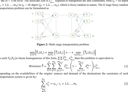
III.Mathematical Formulation

Let us consider a K-stage transportation problem. Also 𝑚𝑚𝑘𝑘 be the number of depots (if k = 1, then if is

terms as origin/ source) of the k−th level and 𝑖𝑖𝑘𝑘be the number of depots (if k = K, then it is called as destination)

of the (k + 1)-th level. The associate cost is 𝑐𝑐̃̂_𝑗𝑗𝑖𝑖_𝑘𝑘+1𝑘𝑘 _{required to transported the unit commodity from}_𝑖𝑖

𝑘𝑘− 𝑡𝑡ℎ depot

(𝑖𝑖𝑘𝑘= 1,2, … ,𝑚𝑚𝑘𝑘) to 𝑗𝑗𝑘𝑘− 𝑡𝑡ℎ depot (𝑗𝑗𝑘𝑘= 1,2, … ,𝑖𝑖𝑘𝑘), which is fuzzy random in nature. The K stage fuzzy random

transportation problem can be formulated as

Figure 2: Multi stage transportation problem

min

𝑋𝑋1∈𝑆𝑆�𝑇𝑇��1(𝑋𝑋1) + min𝑋𝑋2∈𝑆𝑆1�𝑇𝑇��2(𝑋𝑋2)�+⋯+ min𝑋𝑋𝑛𝑛∈𝑆𝑆𝑛𝑛−1�𝑇𝑇��𝐾𝐾(𝑋𝑋𝐾𝐾)��

As each 𝑇𝑇𝑘𝑘(𝑋𝑋𝑘𝑘)is linear homogeneous of this form, ∑ ∑ 𝑐𝑐̃̂𝑗𝑗𝑘𝑘+1

𝑖𝑖𝑘𝑘 _𝑥𝑥

𝑗𝑗𝑘𝑘+1

𝑖𝑖𝑘𝑘 _{then this problem is equivalent to}

𝑀𝑀𝑖𝑖𝑖𝑖𝑖𝑖𝑚𝑚𝑖𝑖𝑀𝑀𝑁𝑁𝑇𝑇��=� � � 𝑐𝑐̃̂_𝑗𝑗𝑖𝑖_𝑘𝑘+1𝑘𝑘

𝑚𝑚𝑘𝑘+1

𝑗𝑗𝑘𝑘+1=1 𝑚𝑚𝑘𝑘

𝑖𝑖𝑘𝑘=1 𝐾𝐾

𝑘𝑘=1

�1− � 𝜆𝜆_𝑖𝑖𝑝𝑝_𝑘𝑘𝑘𝑘−1

𝑚𝑚𝑘𝑘−1

𝑝𝑝𝑘𝑘−1=1

� 𝑥𝑥_𝑗𝑗𝑖𝑖_𝑘𝑘+1𝑘𝑘 ₍₁₎

Depending on the availabilities of the origins/ sources and demand of the destinations the constrains of such transportation system is given by:

� 𝑥𝑥_𝑗𝑗𝑖𝑖₂1 𝑚𝑚2

𝑗𝑗2=1

=𝑎𝑎𝑖𝑖1; 𝑖𝑖1= 1,2, … ,𝑚𝑚1 (2)

� 𝑥𝑥_𝑗𝑗𝑖𝑖_𝐾𝐾𝐾𝐾−1 𝑚𝑚𝐾𝐾

𝑖𝑖𝐾𝐾−1=1

=𝑏𝑏𝑗𝑗𝑘𝑘;𝑗𝑗𝑘𝑘 = 1,2, … ,𝑚𝑚𝐾𝐾 (3)

𝑥𝑥_𝑗𝑗𝑖𝑖_𝑘𝑘𝑘𝑘_≥_0,_∀𝑖𝑖_,_𝑗𝑗₍₄₎

If ∑ 𝑎𝑎𝑖𝑖1 𝑚𝑚1

𝑖𝑖1=1 =∑ 𝑏𝑏𝑗𝑗𝑘𝑘

𝑚𝑚𝑘𝑘+1

𝑗𝑗𝑘𝑘+1=1 , then the problem is said to be balance and constraints (4) is due to the feasibility

condition of the MSTP.

Here, the fuzzy random unit transportation cost denoted as 𝑐𝑐̃̂_𝑗𝑗𝑖𝑖_𝑘𝑘+1𝑘𝑘 _{is of the form}_𝑐𝑐̃̂ 𝑗𝑗𝑘𝑘+1

𝑖𝑖𝑘𝑘 ₌

��𝑐𝑐_𝑗𝑗(_𝑘𝑘1)𝑖𝑖𝑘𝑘_,_𝑐𝑐 𝑗𝑗𝑘𝑘

(2)𝑖𝑖𝑘𝑘_,_𝑐𝑐 𝑗𝑗𝑘𝑘

(3)𝑖𝑖𝑘𝑘_�_,_𝑆𝑆

𝑖𝑖𝑘𝑘𝑆𝑆𝑗𝑗𝑘𝑘� is the set of triangular fuzzy numbers occurred probability 𝑆𝑆𝑖𝑖𝑘𝑘𝑆𝑆𝑗𝑗𝑘𝑘.

Other notation represents, 𝑎𝑎𝑖𝑖1= availabilities of the commodity present for the first state.

(7)

𝑥𝑥_𝑗𝑗𝑖𝑖_𝑘𝑘+1𝑘𝑘 _{= amounts transported from}_𝑖𝑖

𝑘𝑘-th to𝑗𝑗𝑘𝑘+1-th destinations.

𝜆𝜆_𝑖𝑖𝑝𝑝_𝑘𝑘𝑘𝑘−1_{= rate of defective to transport the quantity from}_𝑆𝑆

𝑘𝑘−1interpot to depot 𝑖𝑖𝑘𝑘.

3.1 Recursive Equation for solving dynamic programming problem:

As mentioned above, the dynamic programming technique will be used to convert the multistage problem into a single-stage problem. The recursive equations for the backward dynamic program for the shortest route problem are illustrated in equations (5) and (6). For minimum transportation cost to a certain destination from all the sources at the last stage, is given by the following formula.

Let, for the last stage K, 𝐹𝐹��𝐾𝐾₍_𝑖𝑖

𝐾𝐾−1) =𝑐𝑐̃̂𝑗𝑗𝐾𝐾 𝑖𝑖𝐾𝐾−1_,_𝑖𝑖

𝐾𝐾= 1,2, … ,𝑚𝑚𝐾𝐾𝑖𝑖𝑃𝑃𝐶𝐶𝑎𝑎𝑐𝑐𝑐𝑐𝑗𝑗𝐾𝐾= 2,3, … ,𝑖𝑖𝐾𝐾 (5)

Then calculate 𝐹𝐹��𝑘𝑘₍_𝑖𝑖

𝑘𝑘) = min�𝑐𝑐̃̂𝑗𝑗𝑘𝑘+1

𝑖𝑖𝑘𝑘 ₊_{𝐹𝐹��}𝑘𝑘+1₍_𝑖𝑖

𝑘𝑘)� (6)

𝑖𝑖𝑃𝑃𝐶𝐶𝑖𝑖𝑘𝑘 = 1,2, … ,𝑚𝑚𝑘𝑘 ,𝑗𝑗𝑘𝑘 = 2, … ,𝑖𝑖𝑘𝑘;𝑘𝑘=𝐾𝐾 −1,𝐾𝐾 −2, … ,1

Where

K: number of stages in general, k=1,2,3,...,K 𝑖𝑖𝑘𝑘: the source number at any stage.

𝑗𝑗𝑘𝑘: the destination number at any stage.

𝑚𝑚𝑘𝑘: the total number of sources at stage k.

𝑖𝑖𝑘𝑘: the total number of destinations at stage k.

𝑐𝑐̃̂_𝑗𝑗𝑖𝑖_𝑘𝑘+1𝑘𝑘 _{: fuzzy random transportation cost of stage}_k_{from its sources}_𝑖𝑖

𝑘𝑘to its destination 𝑗𝑗𝑘𝑘+1.

𝐹𝐹��𝑘𝑘₍_𝑖𝑖

𝑘𝑘): fuzzy random optimum value of the studied objective for each source at any stage k.

Therefore, the reduced single-stage transportation problem with fuzzy random cost coefficient are

𝑀𝑀𝑖𝑖𝑖𝑖𝑖𝑖𝑚𝑚𝑖𝑖𝑀𝑀𝑁𝑁𝑍𝑍�̂= � � 𝑑𝑑̃̂_𝑗𝑗𝑖𝑖_𝐾𝐾1 𝑛𝑛𝐾𝐾

𝑗𝑗𝐾𝐾=1 𝑚𝑚1

𝑖𝑖1=1

𝑌𝑌_𝑗𝑗𝑖𝑖_𝐾𝐾1₍₇₎

Where 𝑌𝑌_𝑗𝑗𝑖𝑖_𝐾𝐾1 _{= min{}_𝑥𝑥 𝑗𝑗2

𝑖𝑖1_,_𝑥𝑥 𝑗𝑗3

𝑖𝑖2_{, … ,}_𝑥𝑥 𝑗𝑗𝐾𝐾

𝑖𝑖𝑘𝑘−1_}_and_𝑑𝑑̃̂ 𝑗𝑗𝐾𝐾

𝑖𝑖1_{are calculated through equations (5) and (6) is represented by}

�𝑑𝑑_𝑗𝑗(_𝐾𝐾1)𝑖𝑖1_,_𝑆𝑆 𝑖𝑖

(𝑙𝑙)_�_,_𝑐𝑐_{= 1,2, . . ,}_𝐿𝐿

Model-1: Now, the fuzzy Expectation of (7) is given by

𝐸𝐸 �𝑍𝑍�̂�=� �𝑍𝑍𝑙𝑙+ 4𝑍𝑍₆𝑀𝑀+𝑍𝑍𝑅𝑅�

𝑛𝑛

𝑖𝑖=1

𝑆𝑆𝑖𝑖 (8)

Following the expression of expected value of fuzzy random variable. So, the problem become minimization if 𝐸𝐸 �𝑍𝑍�̂� subject to (2) and (3).

Model-2: The fuzzy variance of (7) is given by

𝑉𝑉𝑎𝑎𝐶𝐶 �𝑍𝑍�̂�=�[𝐸𝐸(𝑍𝑍�̂2₎ 𝑛𝑛

𝑖𝑖=1

− �𝐸𝐸 �𝑍𝑍�̂��2] (𝑌𝑌_𝑗𝑗_𝐾𝐾𝑖𝑖1₎2₍₉₎

The expression of (9) is the variance of fuzzy random variable. So, the problem become minimization if 𝑉𝑉(𝑍𝑍�̂) subject to (2) and (3).

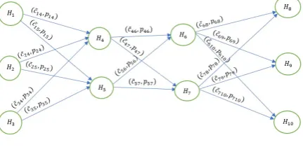
IV.NUMERICAL EXAMPLE

Example-1: Let us consider a 3-stage transportation problem. The availabilities of sources at stage-1 equal are those values of (𝑎𝑎1= 120,𝑎𝑎2= 70 and 𝑎𝑎3= 60). The requirement of the destinations at the last stage are those

values of (𝑏𝑏1= 95,𝑏𝑏2= 103 and 𝑏𝑏3= 52). There are no transportation restrictions on the middle stages

availabilities or requirement.

(8)

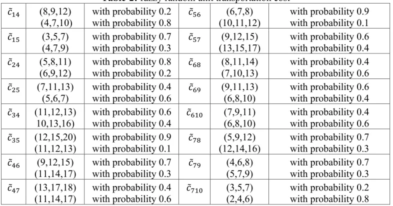
Table-2: fuzzy random unit transportation cost 𝑐𝑐̃14 (8,9,12)

(4,7,10) with probability 0.2 with probability 0.8 𝑐𝑐̃56 (10,11,12) (6,7,8) with probability 0.9 with probability 0.1 𝑐𝑐̃15 (3,5,7)

10,13,16) with probability 0.6 with probability 0.4 𝑐𝑐̃610 (7,9,11) (6,8,10) with probability 0.4 with probability 0.6 𝑐𝑐̃35 (12,15,20)

(11,14,17) with probability 0.4 with probability 0.6 𝑐𝑐̃710 (3,5,7) (2,4,6) with probability 0.2 with probability 0.8

Now we using the dynamic programming problem to convert 3-stage transportation problem to single stage transportation problem and we get the shortest route of the given 3- stage transportation problem.

Table 3: DPP and fuzzy random variable

shortest route fuzzy random cost with probability

𝐻𝐻1− 𝐻𝐻5− 𝐻𝐻7− 𝐻𝐻8 {(17,26,34),0.294},{(24,31,38),0.196},{(21,29,36),0.126}, {(28,34,40),0.084},

{(18,28,36),0.126},{(25,33,40),0.084},{(22,31,38),0.054},{(29,36,42),0.036} 𝐻𝐻2− 𝐻𝐻4− 𝐻𝐻6− 𝐻𝐻8 {(22,31,40),0.224}, {(24,33,42),0.096}, {(21,30,39),0.336}, {(23,32,41),0.144},

{(23,32,41),0.056},{(25,34,43),0.024},{(22,31,40),0.084},{(24,33,42),0.036} 𝐻𝐻3− 𝐻𝐻4− 𝐻𝐻6− 𝐻𝐻8 {(28,35,42),0.168},{(30,37,44),0.072},{(27,34,41),0.252},{(29,36,43),0.108},

{(27,36,45),0.112}, {(29,38,47),0.048},{(26,35,44),0.168},{(28,37,46),0.072} 𝐻𝐻1− 𝐻𝐻5− 𝐻𝐻6− 𝐻𝐻9 {(25,32,38),0.056},{(26,33,39),0.024},{(23,29,37),0.084},{(24,30,39),0.036},

{(21,30,36),0.224}, {(22,31,37),0.096},{(19,27,35),0.336}, {(20,28,37),0.144} 𝐻𝐻1− 𝐻𝐻5− 𝐻𝐻7− 𝐻𝐻9 {(22,29,34),0.216},{(19,26,31),0.144},{(26,33,38),0.024},{(23,30,35),0.016},

{(20,24,28),0.324}, {(17,21,25),0.216},{(24,28,32),0.036}, {(21,25,29),0.024} 𝐻𝐻1− 𝐻𝐻5− 𝐻𝐻7− 𝐻𝐻9 {(24,32,38),0.168},{(25,33,39),0.072},{(22,29,37),0.252},{(23,30,39),0.108},

{(25,34,40),0.112}, {(26,35,41),0.048},{(23,31,39),0.168}, {(24,32,41),0.072} 𝐻𝐻1− 𝐻𝐻5− 𝐻𝐻7− 𝐻𝐻8 {(14,19,24),0.252},{(18,23,28),0.028},{(15,20,25),0.378},{(19,24,29),0.042},

{(15,21,24),0.108},{(19,25,30),0.012)},{(16,22,27),0.162},{(20,26,31),0.018} 𝐻𝐻1− 𝐻𝐻5− 𝐻𝐻7− 𝐻𝐻8 {(18,25,30),0.144},{22,29,34),0.016},{(19,26,31),0.216},{(23,30,35),0.024},

{(16,20,24),0.216}, {(20,24,28),0.024},{(17,21,25),0.324},{(21,25,29),0.036} 𝐻𝐻1− 𝐻𝐻5− 𝐻𝐻7− 𝐻𝐻8 {(23,31,37),0.048},{(21,28,36),0.072},{(22,30,36),0.192},{(20,27,35),0.288},

{(24,33,39),0.032},{(22,30,38),0.048},{(23,32,38),0.128},{(21,29,37),0.192}

All the shortest routes according to their unit transportation cost(which is also a fuzzy random parameters) are shown in the figure

(9)

To find optimal transportation unit at first, we find out the expected cost of each route then the converted transportation problem minimized through Lingo-14.0 subject to the constraints (2) and (3). The optimal solution is

Table 4: Optimum transportation for Model-1

Route Trans. Unit (min) Exp. Value(min) 𝐻𝐻1− 𝐻𝐻5− 𝐻𝐻7− 𝐻𝐻8 0 6554.1

𝐻𝐻2− 𝐻𝐻4− 𝐻𝐻6− 𝐻𝐻8 35

𝐻𝐻3− 𝐻𝐻 4− 𝐻𝐻6− 𝐻𝐻8 60

𝐻𝐻1− 𝐻𝐻 5− 𝐻𝐻6− 𝐻𝐻9 103

𝐻𝐻2− 𝐻𝐻 5− 𝐻𝐻6− 𝐻𝐻9 0

𝐻𝐻3− 𝐻𝐻4− 𝐻𝐻7− 𝐻𝐻9 0

𝐻𝐻1− 𝐻𝐻5− 𝐻𝐻6− 𝐻𝐻10 17

𝐻𝐻2− 𝐻𝐻5− 𝐻𝐻6− 𝐻𝐻10 35

𝐻𝐻3− 𝐻𝐻4− 𝐻𝐻7− 𝐻𝐻10 0

And for model-2:

Table 5: Optimum transportation for Model-2 Route Trans. Unit (min) Var.(min) 𝐻𝐻1− 𝐻𝐻 5− 𝐻𝐻7− 𝐻𝐻8 0 4675.05

𝐻𝐻2− 𝐻𝐻4− 𝐻𝐻6− 𝐻𝐻8 35

𝐻𝐻3− 𝐻𝐻 4− 𝐻𝐻6− 𝐻𝐻8 60

𝐻𝐻1− 𝐻𝐻5− 𝐻𝐻6− 𝐻𝐻9 68

𝐻𝐻2− 𝐻𝐻 5− 𝐻𝐻6− 𝐻𝐻9 35

𝐻𝐻3− 𝐻𝐻4− 𝐻𝐻7− 𝐻𝐻9 0

𝐻𝐻1− 𝐻𝐻 5− 𝐻𝐻6− 𝐻𝐻10 52

𝐻𝐻2− 𝐻𝐻 5− 𝐻𝐻6− 𝐻𝐻10 0

𝐻𝐻3− 𝐻𝐻 4− 𝐻𝐻7− 𝐻𝐻10 0

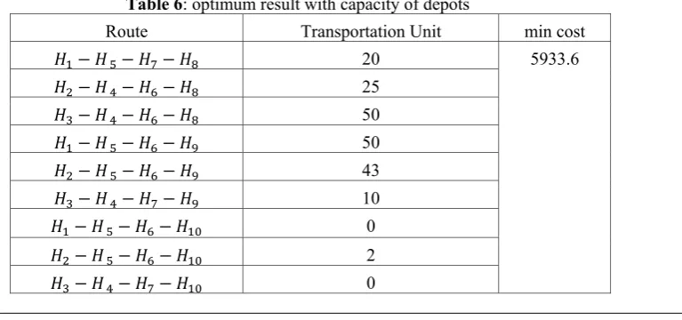
Example-2: Example-2 is similar as example-1, where the internal depots are not in infinite capacity. Instead of that, internal depots have finite capacity of storing. Let the capacity of the depots are

Depots 𝐻𝐻 4 𝐻𝐻 5 𝐻𝐻 5 𝐻𝐻7

Capacity 55 65 50 60 Then the optimal solution is

Table 6: optimum result with capacity of depots

Route Transportation Unit min cost

𝐻𝐻1− 𝐻𝐻 5− 𝐻𝐻7− 𝐻𝐻8 20 5933.6

𝐻𝐻2− 𝐻𝐻4− 𝐻𝐻6− 𝐻𝐻8 25

𝐻𝐻3− 𝐻𝐻 4− 𝐻𝐻6− 𝐻𝐻8 50

𝐻𝐻1− 𝐻𝐻5− 𝐻𝐻6− 𝐻𝐻9 50

𝐻𝐻2− 𝐻𝐻5− 𝐻𝐻6− 𝐻𝐻9 43

𝐻𝐻3− 𝐻𝐻4− 𝐻𝐻7− 𝐻𝐻9 10

𝐻𝐻1− 𝐻𝐻 5− 𝐻𝐻6− 𝐻𝐻10 0

𝐻𝐻2− 𝐻𝐻5− 𝐻𝐻6− 𝐻𝐻10 2

(10)

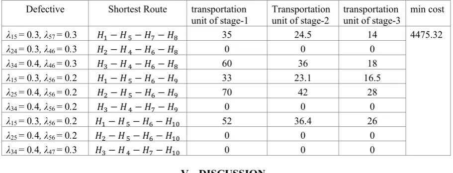
Example-3: Let us consider an example, same as example-1 with the positive defective rate, and corresponding results are

Table 7: Optimum results with defectiveness of the item Defective Shortest Route transportation

unit of stage-1 Transportation unit of stage-2 transportation unit of stage-3 min cost λ15 = 0.3, λ57 = 0.3 𝐻𝐻1− 𝐻𝐻 5− 𝐻𝐻7− 𝐻𝐻8 35 24.5 14 4475.32

λ24 = 0.3, λ46 = 0.3 𝐻𝐻₂− 𝐻𝐻 ₄− 𝐻𝐻₆− 𝐻𝐻₈ 0 0 0

λ34 = 0.4, λ46 = 0.3 𝐻𝐻₃− 𝐻𝐻₄− 𝐻𝐻₆− 𝐻𝐻₈ 60 36 18

λ15 = 0.3, λ56 = 0.2 𝐻𝐻₁− 𝐻𝐻₅− 𝐻𝐻₆− 𝐻𝐻₉ 33 23.1 16.5

λ25 = 0.4, λ56 = 0.2 𝐻𝐻₂− 𝐻𝐻 ₅− 𝐻𝐻₆− 𝐻𝐻₉ 70 42 28

λ34 = 0.4, λ56 = 0.2 𝐻𝐻₃− 𝐻𝐻 ₄− 𝐻𝐻₇− 𝐻𝐻₉ 0 0 0

λ15 = 0.3, λ56 = 0.2 𝐻𝐻₁− 𝐻𝐻₅− 𝐻𝐻₆− 𝐻𝐻₁₀ 52 36.4 26

λ25 = 0.4, λ56 = 0.2 𝐻𝐻2− 𝐻𝐻 5− 𝐻𝐻6− 𝐻𝐻10 0 0 0

λ34 = 0.4, λ47 = 0.3 𝐻𝐻₃− 𝐻𝐻 ₄− 𝐻𝐻₇− 𝐻𝐻₁₀ 0 0 0

V. DISCUSSION

The mathematical form and its numerical illustration help the decision maker to take the following decisions: (i) As these are several paths from an origin 𝐻𝐻1,𝐻𝐻2,𝐻𝐻3 to final destination 𝐻𝐻8,𝐻𝐻9,𝐻𝐻10, the dynamic

programming problem help us to find the path with minimum cost, such paths with their fuzzy random costs are display in table-3. (ii) The optimum results to minimize the expected total cost and variance of total of total cost are shown in Table-4 and Table-5. (iii) Here the optimum paths are non-degenerate in nature and solution are balanced. (iv) It is also seen that in the middle stage 𝐻𝐻7 depots are not used, since to transport the quantity to 𝐻𝐻9

and 𝐻𝐻10through 𝐻𝐻7 gives the more expected cost (31.23, 29.1 respectively) than that through 𝐻𝐻6((22.75.25.06),

(20.51,22.86) respectively). Similarly, when the amount is transport from 𝐻𝐻1 gives the larger value than 𝐻𝐻6. (v)

But, if we assign the capacity of depots then through 𝐻𝐻7 , quantity also transport. In this case the number of

allocations is more than without that of without capacity. (vi) From table-7, it is also seen that if defectiveness of the items is introduced then as expected total transportation amount reduce.

VI.CONCLUSION AND FUTURE RESEARCH WORK

In reality, the last user i.e., retailer shop or seller can’t get the commodity directly from the origin. There may present one or more intermediate depots. So, in general a single stage transportation problem is not realistic in nature. Such a multi stage transportation problem is constructed here. The multi stage problem create multi paths from one origin to one destination. From these multiple available paths unique path is determined here through dynamic programming problem. Here the unit cost terms are taken with vagueness presented by fuzzy random variable, which has been transformed into a deterministic one using expected value of credibility measure of the fuzzy random variable. The model can be extended with solid transportation problem, problem with deteriorating item, model with fixed charge, model with more vehicle cost, etc. Not only that, the similar problem can be formulate and examine with another type of vagueness, like- rough measures, fuzzy rough measures, type-2 fuzzy parameters, etc.

REFERENCES

[1]. A.M. Geoffrion, G.W. Graves, Multi commodity distribution system design by benders decomposition. Manag. Sci. 20, 1974, 822-844.

[2]. A. N. Gani, K.A. Razak, Two Stage Fuzzy Transportation Problem, Journal of Physical Sciences, 10, 2006, 63-69.

[3]. A. Ojha, B. Das, S.K. Mondal and M. Maiti, A transportation problem with fuzzystochastic cost, Applied Mathematical Modelling 38(4), 2014, 1464-1481.

[4]. C. B. Das, Multi-Stage Transportation Problem under Vehicles, Journal of Physical Sciences, 21, 2016,47-61.

[5]. E.E.M. Ellaimony, Different Algorithms for Solving Multi-Stage Transportation Problems, Ph.D., Helwan University, Egypt, 1985. [6]. H.A. Abdelwali, On Parametric Multi-Objective Dynamic Programming with Applications to Automotive Problems, Ph.D., El-Minia

University, Egypt, 1997.

[7]. H. Kwakernaak, Fuzzy random variables-I. Definitions and theorems. Inf. Sci. 15, 1978,129.

[8]. H. Kwakernaak, Fuzzy random variables-II. Algorithms and examples for the discrete case. Inf. Sci. 17, 1979, 253-278.

[9]. I. Berzina, A. Istranikova, The way of solving two-stage transportation problems, Mathematical Methods in Economics, 1999,39 -44. [10]. L.A. Zadeh, Fuzzy sets as a basis for a theory of possibility, Fuzzy Sets and Systems 1(1), 1978,3-28.

[11]. L.A. Zadeh, A theory of approximate reasoning, In Mathematical Frontiers of the Social and Policy Sciences, J. Hayes, D. Michie, and R.M. Thrall (eds.), Cororado, Westview Press, 1979, 69-129.

(11)

[14]. P. Pandian, G. Natarajan, A new algorithm for finding a fuzzy optimal solution for fuzzy transportation problem, Applied Mathematical Sciences, 4,2010,79 – 90.

[15]. S. Malhotra,R. Malhotra, A polynomial Algorithm for a Two Stage TimeMinimizing Transportation Problem. OPSEARCH, 39, 2002,251-266.

[16]. S. Malhotra,R. Malhotra, M.C. Puri, Two Stage Interval Time MinimizingTransportation Problem. ASOR Bulletin. 23, 2004,2-14. [17]. W. Ritha, J. M. Vinotha, Multiobjective Two Stage Fuzzy TransportationProblem. Journal of Physical Sciences 13, 2009,107-120. [18]. Y. Li, P. Jiang, L. Gao and X. Shao, Sequential optimisation and reliability assessment for multidisciplinary design optimisation under

hybrid uncertainty of randomness and fuzziness, Journal of Engineering Design 24(5), 2013,363-382.

Anjana Kuiri.“ An Application of Dynamic Programming Problem in Multi Stage