Node Reproduction Based Range-free
Localization Algorithm in Wireless Sensor
Networks
Xiaoming Wu
School of Information Science & Electric Engineering, Shandong Jiaotong University, Jinan, China Email: [email protected]
Hua Wu, Yang Liu, Jianping Xing, Mingyue Zhao
School of Information Science & Electric Engineering, Shandong Jiaotong University, Jinan, China School of Information Science & Engineering, Shandong University, Jinan, China
Cloud, Computing&communications power management, Texas Instruments, USA Email: [email protected], [email protected], [email protected], [email protected]
Abstract—In this paper, a node self-localization algorithm based on node reproduction (NR) for wireless sensor network (WSN) is proposed. This method is adapted to WSN that anchor nodes present a uniform distribution in three dimensional sensor spaces. During the localization process, by reproducing a 3D special node, which is called the reproduced node, unknown nodes can calculate their own positions automatically. This NR algorithm is a three dimensional range-free approach which does not need extra hardware requests and the unknown nodes can calculate reproduced node by position information from three- different anchor nodes. Finally the unknown position coordinates are obtained by the position information of above four nodes. This approach has low complexity and the localization process is much simpler in simulation. The localization error can also reach a low level compared with classic DV-Hop and Centroid which can be found in simulation and the NR algorithm needs the least localization time. In extreme situations, localization error and time are improved by 25%, 84% and 84%, 88% compared with Centroid and DV-Hop algorithms respectively.
Index Terms—WSN, three dimensional sensing space, node reproduction, self-localization
I. INTRODUCTION
Wireless sensor network (WSN) is an important technology attracting considerable research interest during these years. WSN is composed of thousands of tiny nodes that are deployed in the sensing fields and is widely used in various area, such as intrusion detection, traffic management, space exploration, environmental monitoring, water quality monitoring, precision agriculture design and disaster rescue, etc. Also the advanced hardware design technology have led to the miniaturization of devices which is capable of communication with each other. So these nodes in WSN have limited processing capabilities and energy to be operated. But in these application situations, changing batteries is almost impossible. Meanwhile wireless
sensor network is envisioned to allow for the ease of deployment through redundancy and ad-hoc placement. There are several essential issues in wireless sensor networks. Location estimation is one of the most important subjects. Self-localization capability is such a highly desirable characteristic of WSN.
Until now, WSN localization scheme has been widely researched [1-3], a large amount of which can be found in Reference [4] and [5], but there is yet much work to do in the field. So far two main centralized [6-8] and distributed
[9-11] localization algorithms have been proposed. All the
general localization mechanisms proposed before can be mainly classified as based approaches and range-free approaches. The former approaches determine the node position fully based on distance or angular information acquired using the Time of Arrival (TOA), Angle of Arrival (AOA), Time Difference of Arrival (TDOA), or Received Signal Strength Indicator (RSSI) techniques [12-16]. On the contrary, range-free localization schemes merely rely on the existence of radio connectivity to an existing target instead of measuring distance or angle, which decrease the consumption power and hardware requirements [17-20]. Range-free schemes mainly explore the local network topology and the coordinate computation is derived from the locations of the surrounding anchor node position coordinates [21-24].
information above. NR algorithm requires no specialized range-determining hardware equipped in the sensors, and relies merely on node-anchor communication to localize the unknown nodes. So it can reduce the computation of the whole network. The main task of the unknown nodes is to listen to the packages which are flooded from the anchor nodes in a fixed time slice. So there is no information exchange between neighboring nodes which is more energy and time efficient. Thus the communication overload is decreased and as a result, the lifetime of the whole network will be prolonged.
This paper is organized as following. Part Ⅱ gives some assumptions of the network model and simulation scenarios. The specific implements of NR are listed in section Ⅲ. Analysis of localization performances and future work are given in part Ⅳ and part Ⅴ respectively. Part Ⅵ depicts the conclusions of the whole work.
II. ASSUMPTIONS AND NETWORK MODEL
Some assumptions are made as following. The localization space is supposed to be a cube with the edge length 100m which means the whole volume of the 3D localization space is 100×100×100m3. The anchor nodes are in a uniform distribution in sensing cube which is to say there are 216 anchor nodes in all in the localization space. In some application environments, a part of anchor nodes have to be set into space grids to better explore the surrounding circumstance parameters as illustrated above. Every eight anchor nodes form a cube with the edge length 20m in the space. Unknown nodes are randomly deployed and the number can be changed in this NR method. The other important parameter is the communication range of each unknown node. Once the packages are sent by anchor nodes, enter the communication range of any unknown node, unknown nodes can detect them immediately and record the corresponding anchor information including anchor node ID and the source anchors’ coordinate. In the field where sensor nodes are spread the amount of all sensors are very large. In this way the probabilities that not enough anchor nodes form a cube is very low. Once happens the algorithm will go on but with large deviation. But the algorithm will fail if number of anchors is less than 3.
The reproduced node is supposed to be the center of the cube formed by eight anchor nodes. As said above, there is always a cube whose vertexes are anchor nodes. So in this situation, reproduced nodes must exist in this network.
Ⅲ.REALIZATION OF NRALGORITHM
The core idea of NR algorithm is how to get this reproduced node. This particular process can be found in this part in detail.
A. Definition of Reprodeced Node
In our proposed algorithm, all anchor nodes are supposed to present a uniform distribution in 3D space. Also this sensing space is 100m×100m×100m which means the total number of all anchor nodes is 216. Every
eight anchor nodes can establish a small cube with the length of side 20m as shown in Figure1.
Anchor Node
Reproduced Node
A1
A2
A3
R
A4
A5
A6
A7
A8
20 m
Figure 1. Formation of NR
As shown in Figure 1, Ai (i =1, 2… 8) is an anchor
node with known position coordinates. So once the eight anchor nodes are determined, the reproduced node (Node R in Figure 1) can also be found out. This node is not only the center but also the centroid of the special cube. Of course this node is not a factual sensor node, but just is reproduced in the sensing space to realize localizing in the next step.
Reproduced node is a key node for realizing the whole localization algorithm. The core problem is how to make it. After the node reproduction is finished, unknown nodes can make self-localization by combining three corresponding anchor nodes where reproduced node is derived from. The position determination of NR algorithm is finished by unknown nodes themselves and the process does not consume too much energy which as a result the lifetime of the network is prolonged. The localization process in detail can be seen in the following Part B.
B. Realization of NR Algorithm
information provided in these packages, reproduced node is formed and can be computed. Finally unknown position can be derived using the reproduced node above.
Just as the flowchart shows in Figure 2, first a random fixed time slice T is produced randomly then unknown nodes begin listening to find out whether there are packages entering its communication range in this predetermined time slice T and finally record all the information of three anchor nodes that have sent the most packages. Because three anchors that have sent most packages mean the most nearest to the unknown nodes which can result in least localization error. All the unknown nodes can equally receive packages from all the anchors from the whole network for they are supposed to be the same on the node structure and function. Choosing the three nearest anchors means little localization error. That is because distance error can be accumulated from node to node if too many hops exist.
Start
Set a time threshold T
The time threshold is arrived?
Receive packages from all anchor nodes
YES
NO
Record related information of three anchor nodes that have send the
most packages
Compute the reproduced node based on the recorded anchor node
information
Compute the unknown node coordinates using three anchor
nodes and reproduced node
END
Figure 2. Flow chart of NR algorithm
After the anchor node information is recorded, unknown node begins to analyze that information and finally reproduced node can be determined. Based on the coordinates of three anchor nodes, unknown nodes can deduce a fourth anchor node coordinate that is on the
same plane with the three to make up a square with edge length 20m. This step is to fix a universal plane for deducing reproduced node. After the four anchor nodes (three are detected and the other is deduced) are assured, the center of the square can be determined easily by average coordinate value of them. The difference between this center node and reproduced node is that only one ordinate direction is different and the other two is the same (3D coordinates are composed by three coordinate directions).
By using the center of the square, reproduced node can be computed through adding half of communication range on one of three ordinate directions. But there is a problem in this algorithm. As shown in Figure 3, after the fourth node is determined, we cannot make sure the reproduced node is on which side of the plane. It may be on the same side with unknown node which means low estimation error. However if on the opposite side of the unknown node, it will produce localization error. During our localization, the position of reproduced node on which side is decided randomly and it is not a perfect solution induces lots of uncertainties. But how to solve this problem completely is also a research direction in the future to make better localization accuracy.
Anchor Node Fourth Anchor Node
Center of Plane Reproduced Node
Figure 3. Computation of NR
A1
A3
R
A1
A3
Anchor Node
Reproduced Node
Figure 4. Derivation of unknown node position
In our algorithm, the distances between three anchor
nodes are all the same, which is 20m or 20 2m. Also the distance between reproduced node and three anchors
is 10 3m. If we choose the center of the four known nodes as the unknown position, the error could not larger than 10 3 which means the localization accuracy can be limited below the value above. Simulation results in next part prove this inference.
Ⅳ.ANALYSIS OF LOCALIZATION PERFORMANCE
Here simulations are made in MATLAB software. In MATLAB we first establish a 3D localization space in which unknown nodes are random deployed for easy use. On the contrary, anchor nodes are deployed in 3D grid. Also in this section we present the performance evaluation of NR as well as the comparisons with classic DV-Hop and Centroid algorithms on estimation error and localization time.
A. Self-performance of NR
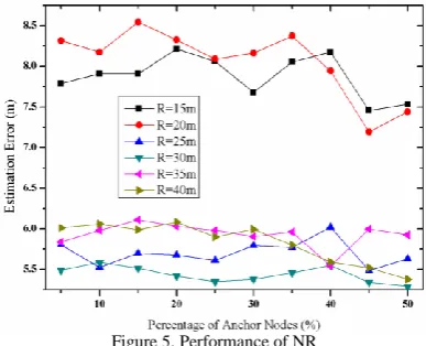
Figure 5 shows the accuracy gain of NR algorithm by changing the number of unknown nodes in order to alter the percentage of all anchor nodes in the 3D sensing space. As Figure 5 shows above, the percentage of anchor nodes changes from 5% to 50% in the sensing space and the estimation error is fluctuating between 5m and 8.5m under six different communication ranges. In the figure we can also find that the effects of anchor node number on the estimation error are so small that the fluctuation range of error is less than 1m. Further the six curves are divided into two obvious parts. When the communication range R is set as 15m and 20m, the estimation error is much larger than that of the other four simulation curves. When communication range R is set as 25m, 30m, 35m, or 40m, the difference is more or less the same. And the fluctuation range is much smaller which is smaller than 2m.
All these performance features are caused by the property of NR itself. Based on finding the special reproduced node, length of communication range for the whole network cover becomes the most critical parameter and the effects of anchor nodes are decreased sharply because in the algorithm their missions are to broadcast beacon information periodically. Also most of the beacon packages from anchors can be sent to unknown nodes efficiently within communication range which assumed in Part Ⅱ. However if the communication range is too small, such as smaller than 10m in the simulating process,
the NR algorithm cannot finish the localization task which is proved by the simulation in MATLAB. That is caused for lower communication range means that it cannot cover the whole sensing space which result the destruction of finding corresponding reproduced node. If so lots of information packages from anchors are lost during the transmission.
Figure 5. Performance of NR
All these performance features are caused by the property of NR itself. Based on finding the special reproduced node, length of communication range for the whole network cover becomes the most critical parameter and the effects of anchor nodes are decreased sharply because in the algorithm their missions are to broadcast beacon information periodically. Also most of the beacon packages from anchors can be sent to unknown nodes efficiently within communication range which is assumed in Part Ⅱ. However if the communication range is too small, smaller than 10m in the simulating process, the NR algorithm cannot finish the localization task which is proved by the simulation in MATLAB. That is caused for lower communication range means it cannot cover the whole sensing space which results the destruction of finding corresponding reproduced node. Lots of information packages from anchors are lost during the transmission.
However, larger communication hardly means high estimation accuracy. As shown in Figure 5, when communication range R is set as 30m, its accuracy is the best. Because the distance between any two anchors is 20m as given in Figure 1, so R=30m means unknown nodes can hear most packages from anchors and the fields where information packages from anchors achieves can increase the cover level of all the localization space. When R is larger than 30m, the packages from different anchors result in confliction which makes some unknown nodes can hear packages which cannot achieve the best situation.
B. Localization Accuracy Comparisons of NR, DV-Hop, Centroid
In this part comparisons of NR algorithm with classic DV-Hop and Centroid algorithms are given.
localization error is the biggest for too many hop counts induce lots of errors. Localization accuracy of DV-Hop totally depends on average hop size of the network which induces lots of uncertainty which results in higher estimation error.
Figure 6. Localization Accuracy Comparisons with R=25m
Figure 7. Localization Accuracy Comparisons with R=30m
Figure 8. Localization Accuracy Comparisons with R=35m
Our proposed NR and Centroid are much closer to some extent. On the whole Centroid is a little better than NR. Their accuracy can both achieve below 0.25R. Especially when R=30m, their errors are below 0.2R. The two algorithms both have much little relationship with number of anchor nodes as analyzed in the last part but they are critical with communication range.
In Figure 8, communication range R is increased to 35m. In this figure, DV-Hop still stands for highest estimation error. However curves of NR and Centroid are almost superposition and all below 0.2R which is caused by large communication range R. Differently in Figure 9, NR is better than Centroid with error as low as 0.15R. So we can find larger communication range under certain of range stands for higher accuracy as also analyzed in last part.
From all the given simulation figures, DV-Hop is the worst on the localization error no matter how the
parameters are changed and always stays at a high level. NR and Centroid are more or less the same on the accuracy. The performances of DV-Hop are totally related to average hop size, hop counts and network size which easily induce a lot of error. When communication range is large enough to 30m, NR will be better than Centroid. So in this situation whole network can be covered completely by beacons from anchor nodes. Packages with information in them from anchors can better enter the scope of unknown nodes and reproduced nodes are determined more accurately which means higher education. In all, all of the three localization algorithms are less affected by anchor nodes which are decided by the inner property of those themselves.
Figure 9. Localization Accuracy Comparisons with R=40m
C. Localization Time Comparisons of NR, DV-Hop, Centroid
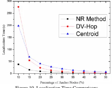
Here we record the average localization time with R=15m, 20m, 25m, 30m, 35m, and 40m of the three respectively. The localization time is a function of percentage of anchor nodes which is shown in Figure 10.
Figure 10. Localization Time Comparisons
reduce time and energy sharply. All in all NR and Centroid is easier in the designing aspect.
We can say our proposed reproduced NR localization algorithm is the most suitable for the rapid positioning situations for there is no complicated computation. So in the future we can think about the use of NR in mobile node scenes in WSN.
Ⅴ.CONCLUSIONS
In this paper, we propose a NR localization algorithm for wireless sensor networks. NR method is a distributed range-free approach which does not require information exchange between neighboring sensors. It has low computation overhead and is simple to implement. NR needs anchor nodes in WSN to flood beacon information periodically which allows each unknown node to record the recording information to realize self-localizing. The estimated position of the unknown node is taken from reproduced node and three other anchor nodes.
Simulation results show NR provides lower localization error than classic DV-Hop and needs little time than DV-Hop, too. Its localization accuracy is similar with that of Centroid algorithm but costs much less time than Centroid which means NR is more suitable for the mutative situations than the other two algorithms in WSN.
REFERENCES
[1] Zhang Youtao, Yang Jun, Li Weijia, Wang Linzhang, Jin Lingling. “An authentication scheme for locating compromised sensor nodes in WSNs,” Journal of Network and Computer Applications, v 33, n 1, p 50-62, January 2010.
[2] Wan Jing; Ghosh, R.K.; Das, Sajal K. “A survey on sensor localization,” Journal of Control Theory and Applications, v 8, n 1, p 2-11, January 2010.
[3] Kulkarni, Raghavendra V; Venayagamoorthy, Ganesh Kumar. “Particle swarm optimization in wireless-sensor networks: A brief survey,” IEEE Transactions on Systems, Man and Cybernetics Part C: Applications and Reviews, v 41, n 2, p 262-267, March 2011.
[4] Kulkarni, Raghavendra V.; Förster, Anna; Venayagamoorthy, Ganesh Kumar. “Computational intelligence in wireless sensor networks: A survey,” IEEE Communications Surveys and Tutorials, v 13, n 1, p 68-96, First Quarter 2011.
[5] S. Gezici. “A survey on wireless position estimation,” Wireless Personal Communications, vol. 44, pp. 263-282, 2008.
[6] G. Mao, B. Fidan, B.D.O. Anderson. “Wireless sensor network localization techniques,” Computer Networks 51 (10) 2529-2553, 2007.
[7] Ding, Yingqiang; Han, Gangtao; Mu, Xiaomin. “A distributed localization algorithm for wireless sensor network based on the two-hop connection relationship”. Source: Journal of Software, v 7, n 7, p 1657-1663, 2012. [8] Erdogan, Ayhan; Coskun, Vedat; Kavak, Adnan. “The
sectoral sweeper scheme for wireless sensor networks: Adaptive antenna array based sensor node management and location estimation,” Wireless Personal Communications, v 39, n 4, p 415-433, December 2006. [9] Chen, Hongwei; Zhang, Chunhua; Zong, Xinlu; Wang,
Chunzhi. “LEACH-G: An optimal cluster-heads selection algorithm based on LEACH”. Source: Journal of Software, v 8, n 10, p 2660-2667, 2013.
[10]Wang, Tsang-Yi; Han, Yunghsiang S.; Varshney, Pramod K.; Chen, Po-Ning. “Distributed aggregate algorithm for average query based on WSN,” Journal on Selected Areas in Communications, v 23, n 4, p 724-733, April 2005. [11]D. Niculescu and B. Nath. “Ad-hoc positioning system,” in
Proc. of IEEE Globecom, San Antonio, TX, Nov. 2001. [12]Chen, Zuo; Chen, Kai. “An improved multi-hop routing
protocol for large-scale wireless sensor network based on merging adjacent clusters”. Source: Journal of Software, v 8, n 8, p 2080-2085, 2013.
[13]J. Caffery Jr. and G.L. Stuer., “Subscriber Location in CDMA Cellular Networks,” IEEE Trans. Vehicular Technology, vol. 47, no. 2, pp. 406-416, May 1998. [14]R. Klukas and M. Fattouche, “Line-of-Sight Angle of
Arrival Estimation in the Outdoor Multipath Environment,” IEEE Trans. Vehicular Technology, vol. 47, no. 1, pp. 342-351, Feb. 1998.
[15]L. Cong and W. Zhuang, “Hybrid TDOA/AOA Mobile User Location for Wideband CDMA Cellular Systems,” IEEE Trans. Wireless Comm., vol. 1, no. 3, pp. 439-447, July 2002.
[16]J. Aspnes, T. Eren, D. Goldenberg, A.S. Morse, W. Whiteley, Y. Yang, B.D.O. Anderson, P. Belhumeur. “A theory of network localization,” IEEE Transactions on Mobile Computing 5 (12) 1663–1678, 2006.
[17]Wang Yun, Wang Xiaodong, Wang Demin, Agrawal Dharma P. “Range-free localization using expected hop progress in wireless sensor networks,” IEEE Transactions on Parallel and Distributed Systems, v 20, n 10, p 1540-1552, 2009.
[18]Li Mo, Kowloon, Liu Yunhao. “Rendered path: Range-free localization in anisotropic sensor networks with holes,” IEEE/ACM Transactions on Networking, v 18, n 1, p 320-332, February 2010.
[19]Chan, Yiu Wing Edwin; Soong, Boon Hee. “A new lower bound on range-free localization algorithms in wireless sensor networks,” IEEE Communications Letters, v 15, n 1, p 16-18, January 2011.
[20]Wang, Sheng-Shih; Shih, Kuei-Ping; Chang, Chih-Yung. “Distributed direction-based localization in wireless sensor networks,” Computer Communications, v 30, n 6, p 1424-1439, March 26, 2007
[21]A. Savvides, W.L. Garber, R.L. Moses, M.B. Srivastava. “An analysis of error inducing parameters in multihop sensor node localization,” IEEE Transactions on Mobile Computing 4 (6) 567–577, 2005.
[22]F.K.W. Chan, H.C. So, “Efficient weighted multidimensional scaling for wireless sensor network localization,” IEEE Transactions on Signal Processing 57 (11) 4548–4553, 2009.
[23]J.A. Costa, N. Patwari, A.O. Hero. “Distributed weighted-multidimensional scaling for node localization in sensor networks,” ACM Transactions on Sensor Networks 2 (1) 39–64, 2006.