Cluster-based Three-dimensional Localization Algorithm for Large Scale Wireless Sensor Networks

Cluster-based Three-dimensional Localization

Algorithm for Large Scale Wireless Sensor

Networks

Jian Shu

School of Computing, Nanchang Hangkong University, Nanchang, P.R.China [email protected]

Ronglei Zhang, Linlan Liu, Zhenhua Wu and Zhiping Zhou School of Computing,Nanchang Hangkong University, Nanchang, P.R.China {[email protected], [email protected], [email protected], [email protected]}

Abstract—In wireless sensor networks, three-dimensional localization is important for applications. It becomes a challenge with the scale of network getting large. This paper proposes a three-dimensional localization algorithm for large scale WSN on the basis of cluster. Focusing on the MDS-based localization, it adopts the cluster structure and the global coordinate system to represent the whole network logically, and reduces the influence of range measurement errors through decreasing the probability of multi-hop. With the combination of variable power of nodes and the triangle principle, the range measurement errors can be corrected. Through the comparison of three different computations in the algorithm of simulations, correction effects are presented. To address the proposed algorithm, CBLALS, more convincible, the comparison of CBLALS and DV-Distance (3D) is taken. The result shows that the positioning accuracy of CBLALS is much better than the one of DV-Distance (3D). With the increasing of the range measurement error, the positioning error of CBLALS varies gently, and could be controlled within 55% while the range measurement error is 30%.

Index Terms—Wireless Sensor Networks,Three-dimensional Localization, Multidimensional Scaling

I. INTRODUCTION

The localization problem for wireless sensor networks itself is a hot issue in current studies. In most applications, acquiring the position information of sensor nodes is indispensable. For example, in military field, WSN is used to collect and spy the comprehensive information of the battlefield; In civil field, WSN is used to prevent forest fire, to monitor the environment and to track the target etc; In these applications, the information is meaningful when node position is acquired. Normally, the nodes are deployed in actual environment which is unpredictable; only having the two-dimensional coordinate of a node can not exactly depict where a node is. Therefore, it is

necessary to position the nodes in three-dimensional space.

The early localization algorithms for WSN focus on researching and innovating in the basic theories. There is a lot of valuable papers on localization algorithm appeared in this stage. Localization algorithms are falling into two categories--Range-based and Range-free [1], according to that the range between two nodes is measured or not. Among that, the range-based algorithms, such as RSSI, TDOA and AOA [2], take some range measurement methods to get the range estimation between an unknown node and an achieved node or an unknown node and a beacon node. Then trilateration method, multilateration method or least square method are employed to compute the unknown node coordinate in two or three dimensional. There are two ways to obtain the unknown node coordinate. The first one is that all nodes communicate with beacons directly, and the range between them is estimated. Their coordinate is computed immediately when enough distance information is achieved. The second one is that nodes with known coordinate are promoted to be beacon nodes, or they are assigned with weights, and node coordinate is computed by flooding over the networks. The range-free localization algorithms do not measure the range between nodes directly, or do not measure the range at all. Position is determined by hops and geometry information between beacons, as well as between an unknown node and a beacon in the case of two-dimensional positioning. For example, DV-Hop employs distance vector routing protocol to obtain the distance between an unknown node and a beacon. It is similar to Amorphous [3, 4]. And what is more, HEAP [5], APIT [6] and Convex programming algorithm [7] estimate the unknown node position with Centroid algorithm directly or indirectly. In addition, there are some un-normal localization methods, such as MDS-MAP algorithm [8] based on multidimensional scaling technique and the scene analysis technology in Microsoft’s RADAR system [9]. These methods can be applied in both range-based and range-free.

This paper is sponsored by National Nature Science Foundation

The requirements for localization algorithm are different in applications. Range-based algorithm could reach a higher precision than range-free algorithm. But it depends more on the accuracy of the range measurement between nodes, and it leads to errors of non line-of-sight brought by the interference of obstacles and other environmental problem. What is more, nodes need additional hardware facilities to do the range measurement. For example, when the range is measured by the following methods: RSS attenuation, ultrasonic and infrared ray, it will cause reflection, refraction or the multi-path effect for wireless signals, if there are obstacles between nodes. As a result, the obtained range gravely deviates from theory. The range-free localization algorithms do not measure the distance between nodes directly, but their performances are closely relevant to the amount of beacons, the density of nodes, and the connectivity of networks. For example, only if the average connectivity is at 10 and beacon ratio is at 10% in an isotropic network, can the positioning accuracy of DV-Hop reach 33% [10].

With the improvement of the localization theory, the studies on localization algorithms focus on the following aspects. The first one is how to refine the precision of localization algorithm or how to reduce the position error. [11] and [12] propose a neighbor collaboration method, with which the position process is divided into two stages-- initial stage and iteration refinement stage. At initial stage, the rough coordinate of nodes is computed. At iteration refinement stage, each node communicates with the neighbors, re-computes and updates the position of themselves according to the neighbor coordinate as well as the range between the node and their neighbors, and repeats the process until the iteration is ended. The second one is to propose a new method combining two or three different localization algorithms or some special localization methods. For example, [13] proposes a new localization algorithm with the combination of the merits of two different localization algorithms. At beginning, it applies Bounding Box [14] method to obtain rough coordinate of the unknown nodes. As a distributed algorithm, Bounding Box method has lower computational complexity and efficient coverage speed. However, with the decreasing of beacon density, the position accuracy will dramatically reduce. Trilateration or multilateration method can acquire higher accuracy even with fewer beacons. Therefore, the author proposes a new localization algorithm with the combination of Bounding Box method and improved multilateration method. [15] applies mobile beacons in locating unknown nodes, in which it uses some mobile beacons to cover a location area, and employs the RSSI, received from the mobile beacons, to position the unknown nodes. The third one is to improve or extend the existing localization algorithms. [16] proposes a three-dimensional localization algorithm(APIT-3D) based on APIT. It determines if an unknown node is in a tetrahedron which has four known nodes. And then, it takes the centroid of the tetrahedron as the estimated position of the unknown node. [17] proposes a distributed localization algorithm based on the centroid method. The algorithm uses three-dimensional auxiliary

coordinate system to establish the constraints on communication and the geometric relationships between nodes. With the determination of the multiple sides and the curved surface of a 3d-body, a 3d-body is constructed. Then the centroid is taken as the estimated position of the unknown node.

All these localization algorithms mentioned above haven’t cared about the three-dimensional localization problem for large-scale WSN yet. When the scale of network gets large, it is a challenge to improve the stability and robustness of the localization algorithm. This paper proposes a cluster-based three-dimensional localization algorithm for large scale wireless sensor networks (named CBLALS for short), which is based on range. Firstly, it improves tri-colors method, which uses this method to establish cluster for the whole network and applies the three-dimensional localization for each cluster. Secondly, it picks some nodes in a cluster according to certain rules to establish the global coordinate system. Finally, the local coordinate of each cluster is transformed to global coordinate by CH (cluster head). With the combination of the triangle principle and the variable power levels of nodes, a method is proposed to correct the range measurement error between nodes and to improve the accuracy of position.

II.RELATED PROBLEMS

The localization algorithms for WSN are divided into centralized computation and distributed computation. The former usually transmits all the information required to Sink or back end, where coordinate for unknown nodes is computed. The advantage of this computation is that there are no limits of the costs on computation and storage. The disadvantage is that all nodes in the network need to send position information to Sink or back end. When the scale of networks gets large, the nodes near Sink may lead to heavy communication or message congestion. As a result, the other nodes may be difficult to contact with Sink, and would not finish the position process. The later is different from the former in that all nodes take part in computing its coordinate. Even though the accuracy is lower than the centralized computation, the network communication overhead is greatly reduced, especially for large scale WSN.

With the topological control method, the network can be logically divided into small area，which is cluster. Local position in each cluster is conducted, and then the local coordinate in each cluster is transformed to the global coordinate system. Through the cluster topological, centralized computation of the localization algorithm can be changed into distributed one.

rang-based with 5% range measurement error, when the number of nodes in network is 200, the number of beacon nodes is 4, and the average connectivity of node is 12.1. So, the accuracy is better considerable in range-based.

A. The MDS- based localizaiton process

MDS is a method of data analysis. It builds the dissimilarity matrix to analyze the difference between objects. The dissimilarity matrix varies with the change of research on objects. When the dissimilarity between objects is the corresponding Euclidean distance, it can be depicted by both Metric MDS and Non-metric MDS [18] through 2D or 3D coordinate. The algorithm based on MDS takes nodes as objects, collects the range information between nodes to construct the dissimilarity matrix, and then computes the coordinate of unknown nodes.

The difference between Metric MDS and Non-metric MDS is whether the real range measurement between the nodes is known. The paper, based on metric MDS algorithm, does not take Non-metric MDS into account. The localization algorithm based on Metric MDS (MDS for short) usually includes the following steps [19]:

1) Determine the Stress function. In the process of positioning for WSN, the obtained range measurement always includes errors. Consequently, the coordinate by the MDS algorithm also has these errors. The goal of the algorithm does not require the absolutely precise of coordinate, but to meet the Stress function through multiple iterative steps. This paper takes kruskal Stress [20] to define the Stress function:

( )

(

)

∑

<

− =

j i

ij ij ij

r X w d X

2 )

( δ

σ ⑴

Where d ij

( )

X is the distance matrix, δij is the

dissimilarity matrix, and

w

_ijis the weight which is set to

1 or 0, according to whether the corresponding range is obtained.

2) Construct dissimilarity matrix. all range information between nodes is collected to construct dissimilarity matrix where the elements are the squared range between the corresponding nodes.

3) Apply MDS algorithm in the dissimilarity matrix to compute the coordinate for nodes. First, the dissimilarity matrix is double centered with formula ⑵:

T

n

n HD H XX

B _× = − 2 =

2

1 ⑵

Where D2 is the dissimilarity matrix,

e e I

Hn×n = n×n− 1_n T is the centered matrix,

I

n×nis the

unit matrix e1×n =[1,1,...,1] . Second, eigenvalue

decomposition is applied in

B

_n×n, and then the largest three eigenvalues and their corresponding eigenvectors are reserved. Finally, the coordinate matrix is computed with formula ⑶:

2 1

UV

X = ⑶ Where matrix U is composed of three column

vectors-

u

₁,

u

₂,

u

₃, and each vector- 2 1

1

v

, 2 1

2

v

, 2 1

3

v

is the main diagonal element of matrix V , other elements

of matrix V are 0, thus, matrix X is three-dimensional matrix for reference system of nodes.

III. CBLALS ALGORITHM

According to the MDS-based localization algorithm and the requirement of positioning for large scale WSN, CBLALS localization algorithm utilizes cluster topology to divide the whole network into small clusters. In each cluster, MDS algorithm is applied to compute the in-cluster relative coordinate.

From section II mentioned above, it is known that the accuracy of positioning and the accuracy of range measurement are related closely. That is, the more accuracy of range measurement between nodes is achieved, the more accuracy of nodes position is achieved. Usually, by using RSS experience attenuation model, the distance between the send node and the receive node can be estimated through statistic of signal propagation loss. [21] has taken the location engine provide by CC2431 chips, manufactured by TI Company, to esteblish a test bed for position system. Some experiments have already done with the test bed. The location engine of CC2431 also used RSS experience attenuation model [22] to do the range measurement. CBLALS takes this RSS model as well.

When taking RSS experience attenuation model to estimate the range, [23] points out that the attenuation follows the lognormality experience model, but there are many factors infacting the parameters in the model. It proposed a curve fitting method to work out the function between distance and receiving power. Through a lot of experiments, it reached a conclusion that the range measurement accuracy is higher when distance is shorter. WSN is essentially a multi-hop network. MDS-based localization algorithm utilizes RSS experience attenuation model to estimate the range between nodes. It is inevitable to estimate multi-hop distance to be measured. With the coverage area and the denstiy of nodes getting change, it cannot solve the problems radically to increast the send power of nodes. Thus, the normal solution is to search the shortest path between two nodes. All of one hop distance of the path is accumulated as the estimation of multi-hop distance. Therefore the measurment error of the multi-hop distance is inversely proportional to the density of nodes and the connectivity of network. It is also found that the more hops between nodes, the more error to the measurment range. Employing culster to divide the network can not only reduce communication costs, but also decreace the complexity of the computation. Besides, the structure of cluster can also dramatically reduce the multi-hop in dissimilarity matrix, and improve the overall range measurment accuracy.

A. The improvement of the tri-color algorithm

gray. All nodes in white state are at beginning. Then, Sink node launches clustering command, and marks itself black. A white node changes itself to gray when it received a massage from a black node and waiting for a period of time, which is inversely proportional to the distance between itself to the black node. It is simliar that when a white node received the massage from a gray node, the wating time is also inversely proportional to the distance from itself to the gray node. During the actual clustering process, it is difficult to acquire the accurate distance between a white node and a black node or even a gray node. So it is possible to cause massage conflict which will lead to bad clustering effect. The paper improves the tri-color method through using the signal strength loss, instead of the distance. Assume that each node has an exclusive global ID. Formula ⑷ is employed to compute the waiting time.

( )

ID c

LOSS a

T b

w = ⋅ + ⋅log10

⑷

Where T_i is the waiting time, LOSS is the loss of

received signal strength (RSS),

a

，

b

and

c

are the control parameters which can be set for experiments.

B. The process of CBLALS

CBLALS assumes that all nodes can send massages with different power, which are randomly deployed in three-dimensional space. The steps of CBLALS are as follows:

1) All nodes keep in listening state, when they are deployed. Then Sink node launches clustering message to create clusters, according to the improved tri-color method.

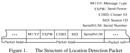
2) Each cluster has different range measurement cycle to estimate the range between in-cluster nodes. Range measurement starts with one cluster by another. For each cluster, the process of range measurement is controlled by CH. In clustering process, CH has already stored all in-cluster node IDs. CH set its ID as cluster ID. Based on in-cluster node IDs, a range measurement queue is created by CH. And it starts to send location detection packets, which are composed of message type, send power level, cluster ID, source ID and serial number, as show in figure 1:

Figure 1. The Structure of Location Detection Packet

Nodes in cluster receive the packets and determine if the packets belong to the corresponding cluster. If they are assured, the receiving nodes begin the sampling period to acquire RSSI of the sampling packets. Each receiving node maintains a local range measurement result table. After the sampling period, the average receive signal strength loss is computed for different power levels, and is put to the corresponding result table. If there is no value of loss, then zero is set to the corresponding element in table.

The receiving nodes send the tables back to CH with the packet structure shown in figure 2:

Figure 2. the packet structure of local range measurement results

Finally, after the CH receives the range measurement results, it will take node ID from the range measurement queue, the range of which is to be measured. That is, the next measurement is started. Otherwise the CH will repeat the current range measurement period until it receives the results table of current period.

3) CH begins to correct the range measurement errors after receiving all range measurement results. Suppose that the send power

Pt

_i has

k

levels, the radius of communication is R_icorresponding to the power levels, where i =1,2,3,..., k . The different radius of

communication can be obtained from the hardware specifications or from the experiments. Suppose a cluster has

m

members for each power level, CH constructs the dissimilarity matrix by converting the received signal strength loss to distance using the RSS experience attenuation model. The dissimilarity matrix in the ith power level is shown in table 1:

TABLE I. THE DISSIMILARITY MATRIX IN I-TH POWER LEVEL

12

d d13 d1m 21

d

23

d d2m m

d3 31

d d32 1 m

d dm2 dm3

Therefore, a pair of nodes may have two distance measurement values; due to the asymmetry of link quality caused by the different environment of two measurement processes. CBLALS takes the mean of two distance measurement values as the final result.

For each dissimilarity matrix of different power levels, CBLALS uses triangle principle to correct the distance measurement errors, according to the following steps:

According to the triangle principle, the relationships of d12, d13 and d23 are checked. Determine the other inequalities in the way above, namely uses formal ⑸ for each possible triangle according to a power level:

( )

( )

( )

⎪ ⎪ ⎪ ⎪

⎩ ⎪⎪ ⎪ ⎪

⎨ ⎧

> +

> +

> +

< +

< −

< −

st tr sr

tr sr st

sr tr st

st tr sr

tr sr st

sr tr st

d d d

d d d

d d d

d d d

d d d

d d d

| |

| |

| |

⑸

If the six inequalities in formal ⑸ are ture, it is

assured that the distance measurement of

d

₁₂,

d

₁₃and

d

₂₃

and the reliability of each distance i

C12,

i

C13 and

i

C23

is set to 1.

If any inequalities in formal ⑸ are not true, for example,

(

d₁₂ + d₂₃

)

< d₁₃ , it is implied that there must

be an inaccurate distance in the inequalities at least. In this state, firstly, set the reliability of one distance to 0. For example, set the reliability ( i

C₁₃) of the distance (d₁₃) to 0, then the reliabilities of the other two distances can be both set to 1. It should be determined again for distance

13

d

to see if there exists an available triangle constraint in dissimilarity matrix at each power level, and the corresponding reliability is set to 0 or 1. If there is no available triangle restrain, then for other two distances (d₁₂ and d₂₃ ) in the inequality, their reliability is determined in the same process. If the reliability of the two distances can be confirmed as 1 after the determination process, it can be proved that the measurement distance of

d

₁₃ has an error. Therefore, for the error-distance ( d₁₃ ), the value is increased or

decreased to meet the formal ⑸ under the constraint of the communication radius. The process above is repeated to find a proper value.

Otherwise, if the reliability of the two distances (d12

and

d

₂₃) is 0 or at least one of them is 0, it is concluded that all the three distances can not be corrected by the triangle principle. The only constraint to the distances is the communication radius at different power levels. Two boundary power levels for each error distance are found out by searching the entire available dissimilarity matrix, and re-calculate the distance using formal ⑹ as follows:

i j i R R R d − ⋅ +

= α 1 ⑹

Where, j

R and Ri (

i

<

j

) are the boundary power

levels. Only if the power level is lowest, there isRj = 0,

α

is the control parameter. The reliability of the corresponding distance can be set in actual situation.

Finally, the errors for all elements are corrected in the dissimilarity matrix using the same method. Then the value of reliability is multiplied by the value of distance as the final result for the dissimilarity matrix.

4) For each final dissimilarity matrix, the MDS algorithm is applied to compute the in-cluster relative three-dimensional coordinate, and the coordinate matrix is created by CH.

5) The global coordinate conversion is conducted after all in-cluster relative coordinate is computed. On the basis of coordinate system, it can be performed for three dimensions as long as four points are not in a plain, whose coordinate is known in both systems. Therefore when the in-cluster relative coordinate matrix is established, each CH starts to pick four nodes to construct global coordinate system. In order to increase the accuracy of the transformation, CH must assure that the distance between the picked nodes is as long as possible.

After that, Sink or back end also generates a range measurement queue which consists of all CH IDs. Each CH uses the backbone built in the process of cluster construction to estimate the distance, and the distance is computed by the accumulation of the one-hop distance, which is the least path between the picked nodes from one cluster to another. CH stores the range estimation results, and sends them back to Sink or back end. Sink or back end operates the process of transformation, and sends the transfer variables back to CH. Finally the global coordinate of the in-cluster nodes is achieved by the CH.

CBLALS transforms the local relative coordinate of nodes to the global coordinate system by the method proposed in [25], which is named Horn method for short in the following sections. Horn method uses the canonical least error to define the transformation error; as the picked nodes are used to compute only, the speed is faster. The goal of Horn method is to find the translation variables which are a scale variable, a transform variable and a rotation matrix that transform nodes in local coordinate system to the global coordinate system using the formal ⑺ as follow:

t sRx

x_G = _L + ⑺

Where

x

_G is the global coordinate and

x

_L is the local relative coordinate,

s

is the scale variable,

t

is the transform variable, and R is the rotation matrix.

Horn method approaches this problem using mean square deviation; it is to find transformation variable using formal ⑻ as follows:

∑ = = n i i R s t e R s t 1 2 , , || || ) , ,

( _{arg min} ⑻

Where e_i = x_G|i −SRx_L|i−t .The specific steps of

the method are as follows:

a) Compute the centroid of x_G|_i and xL|i. Then shift

them with respect to the centroid as formal ⑼:

⎩ ⎨ ⎧ − = ′ − = ′ L i G i L G i G i G x x x x x x | | | | ⑼

Where

_∑

= = n i i G G x n x 1 | 1 _,

∑

= = n i i L L x n x 1 | 1 _.

b) Use formal ⑽ to compute scale variable

s

as follows: 2 1 2 1 | 2 1 | || || || || ⎟⎟ ⎟ ⎟ ⎟ ⎠ ⎞ ⎜⎜ ⎜ ⎜ ⎜ ⎝ ⎛ ′ ′ =

∑

∑

= = n i i L n i i G x x s ⑽

c) Use formal ⑾ to compute M .

( )

∑

= ′ ′ = n i T i L i G x x M 1 | | ⑾

Compute the eigenvalue decomposition of M TM _.

That is, eigenvalues

λ

₁,

λ

₂,

λ

₃ and eigevectors

u

ˆ

₁,

u

ˆ

₂,

3

ˆ

u

have to be found out. Then the rotation matrix

R

is as formal ⑿:

⎟ ⎟ ⎠ ⎞ ⎜ ⎜ ⎝ ⎛ + + =

= − T T T

u u u u u u M MS

R 3 3

3 2 2 2 1 1 1

1 1 _{ˆ ˆ} 1 _{ˆ ˆ} 1 _{ˆ ˆ}

λ λ

λ

d) The scale and the rotation matrix are acquired by formal ⑽ and ⑿, then the formal ⒀ is employed to compute

t

:

L G sRx

x

t = − ⒀ e) Finally each CH uses formal ⑺ to compute the global coordinate for other nodes in their cluster.

IV. SIMULATION RESULTS

In order to validate and analyze the proposed three-dimensional localization algorithm (CBLALS), the paper uses Matlab to simulate. The configuration and deployment of the experiments are as follows: there are about 1,500 sensor nodes deployed in 100×100×100 space by random uniform distribution. Each node can send location detection packets in 8 different power levels.

This paper has already done the experiments on nodes to validate the improved tri-color algorithm, in which 15 nodes are deployed in a corridor, three or four clusters are established in each experiment, and the number of nodes is nearly the same. Because the clustering algorithm is not the primary issue the paper addresses, it is not discussed in detail. In this paper the clusters are created by simulating.

To obtain the topology of the network whose distribution is uniform and random, it is assumed that all nodes communicate with the lowest power level at the initial stage. To create a uniform network, the following method is taken. Arbitrary coordinate is assigned as the first node position. n nodes, n is 20000 in the simulation, are created uniformly in a sphere which center is the first node. A node is taken as the center of the second sphere to be created, which is picked up randomly from n. Similarly, n nodes are created in the second sphere. The way is repeated 59 times. The backbone is constructed by centers coming from spheres. Nodes in clusters are picked up from each sphere. A uniform network is established. The first center is chosen to be a CH, then the second center is supposed to be a relay node, and the third center must be another CH, and so on. After that, 48 positions are chosen as its in-cluster member nodes randomly in the covered area of each CH. Seen from the statistics, it can be found that most nodes have about 10~15 neighbors except the nodes which are on the edges of the network. The result shows that the establishment of the cluster is ideal.

The initial coordinate of all nodes is obtained after the establishment of the network. As the initial node coordinate is supposed to be accurate, the simulation uses them as the reference to evaluate the proposed algorithm.

According to the CBLALS, the coordinate of the nodes is computed with range measurement error at 5%, 10%, 15%, 20%, 25% and 30%. Three different computations of the nodes coordinate are applied in the simulation experiments. For the first time, the correction method for range measurement error is not used; for the second time, the correction method to restrict the range measurement errors is used. For the third time, 10% beacons are used to correct the range measurement errors. The three times computations are denoted as CBLALS (1), CBLALS (2) and CBLALS (3) respectively. Figure 3

shows the average positioning accuracy with the increasing range measurement error:

Figure 3. the position error in three different computations

Figure 3 shows that the obtained position errors are very close and less in three different computations when the error of the range measurement is less than 10%. And the positioning is more accurate. With the increasing error of range measurement, the position error can be controlled by the range error correction method. The position accuracy can be obviously improved with CBLALS (3).

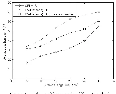
To evaluate CBLALS algorithm more convincingly, the simulation experiments DV-Distance (3D) and the range error corrected DV-Distance (3D) are attended in comparison. It is assumed that the density of the beacons is 10%, and the distribution is uniform in the network. The connectivity of the networks is 10~15. The result is shown as figure 4.

Figure 4. the position error in different methods

In DV-Distance (3D), the unknown nodes position is computed with multilateration method. The accuracy of the position error is about 34%, even though the range measurement is only 5%. With the increasing range error, the position error increases rapidly. But after the range error correction process proposed in this paper is taken, the position error is reduced a lot. With the comparison of the two localization algorithms, it can be easily found that the accuracy of positioning by CBLALS is much better than DV-Distance (3D). CBLALS can eventually control the position error at 55% even with 30% range error.

global coordinate system to achieve the global coordinate of the whole network. At last the global coordinate is transformed in each cluster. It can be seen that the achieved global coordinate and the final positioning accuracy of nodes are interrelated closely, and the accuracy of global coordinate depends on the estimate of the multi-hop distance between nodes in a cluster. With the computation of the global coordinate based on MDS algorithm, the one-hop distance between the chose nodes in a cluster can be utilized furthest to improve the accuracy of transformation. In order to show the establishment of the global coordinate system and the capability of transformation, the comparison between the proposed method in this paper and the ABC algorithm [26] is made in the experiment.

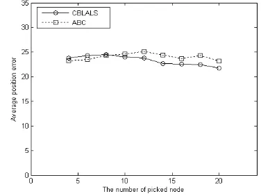
Three anchor nodes of the whole network are chosen randomly, and the plane determined by the three anchor nodes is considered as the XOY-plane of dimensional coordinate system in ABC algorithm. According to the transforming rule of coordinate system, a certain amount of nodes are chosen to be concerned with establishing the global coordinate system in each cluster, and the corresponding global coordinate is computed. Among that, the multi-hop distance between the chosen node and the anchor node is also achieved by the accumulation of the one-hop distance in the shortest path. Finally, according to the computed coordinate of the chosen nodes, the transforming variables of global coordinate and the global coordinate of other nodes in the network are computed. The average range measurement error of network is set to 10%, and the connectivity of the network is 10~15. Figure 5 shows the relationship of average positioning error and the number of nodes chosen to build global coordinate in the case of CBLALS algorithm and ABC algorithm respectively.

Figure 5. the position error with the estebilished global coordinate system of different algorithm

It can be seen from the figure that the average positioning errors achieved with two algorithms are very close when the number of nodes is less than 10. However, with the increasing amount of nodes which are chosen to be concerned with establishing the global coordinate system in a cluster, the average positioning errors with CBLALS algorithm are less than the one with ABC algorithm. This is because CBLALS algorithm takes use of one hop distance more than ABC algorithm does, so

that the distance estimation of CBLALS is more accurate. Therefore, the positioning accuracy of CBLALS is improved.

V.CONCLUSIONS

The network is divided twice logically by the proposed CBLALS algorithm. Cluster structure is used for the first time, and global coordinate system is used for the second time. For each cluster, MDS algorithm is employed to compute the local relative coordinate, and RSS experience attenuation model is used to estimate the distance between nodes. When establishing global coordinate, four nodes for each cluster are picked up to establish the global coordinate system, and then the transform variables are computed. After that, each CH uses the transform variables to compute the global coordinate for each in-cluster node.

The using of cluster structure can reduce the existing possibility of multi-hop distance which is the main obstruction for the MDS algorithm. And with the range error correction method, the accuracy of position is obviously improved. The two logically divided processes can also effectively reduce the communication costs, because the communication in each cluster is often one hop and for the entire network only CH needs to communicate with multi-hop.

It is necessary to study on range measurement in future, because the performance of localization algorithm depends much on the accuracy of range measurement (except a range-free localization algorithm). In real environment, the using of RSS experience attenuation model to estimate the distance may be interfered by environments, especially in three-dimensional situation. For example, the receiving signal loss is much different even though nodes are in the same distance of different height. Moreover, the non-line-of-sight to the distance measurement is also a challenge to deal with.

Besides, the estimation of the multi-hop distance in the positioning of the wireless sensor network becomes another issue. The distance achieved by the accumulation of the one-hop distance in the shortest path and the connectivity of the network are related closely with the deployment of network. In this algorithm, the number of hops can be reduced by employing the cluster structure, so as to achieve more accurate range measurement. In the transforming of the global coordinate, the estimation of the multi-hop distance also exists, which will impact the positioning accuracy. In the three-dimensional positioning, the errors affect positioning accuracy more. Therefore, the method that reducing the errors of the multi-hop distance needs to be further researched on in the future.

VI. REFERENCE

[1] He Tao, Huang C, Blum B M et al. Range-free localization schemes for large scale sensor networks: Proc 9th Annual Int’1 MobiCom 2003 [C], [s.n.],[S.l.],2003.

[3] NICULESCU D,NATH B. Dv-based positioning in ad hoc networks [J]. Kluwer journal of Telecommunication System,2003,22(1): 267~280.

[4] NICULESCU D, NATH B. Ad hoc positioning

system(APS): Global Telecommunications Conference 2001 [C], [s.n.] , [S.l.] , 2001.

[5] Bulusu B, Heidemann J, Estrin D. Density adaptive algorithms for beacon placement in wireless sensor networks. In: IEEE ICDCS’01,Phoenix, AZ. April 2001. [6] NAGPAL R. Organizing a global coordinate system from

local information on an amprophous compute [DB], AI Memo 1666, MIT AI Laboratory. 1999.

[7] Doherty L, Pister KSJ, Ghaoui LE. Convex position estimation in wireless sensor networks. In: Proc. Of IEEE INFOCOM 2001, vol.3, Anchorage: IEEE Computer and communications Societies, 2001, 1655~1663.

[8] YI SHANG,WHEELER R. ,YING ZHANG. Localization from Mere Connectivity: ACM International Symposium on Mobile Ad Hoc Networking & Computing, 2003 [C], [s.n.] , [S.l.] ,2003.

[9] Bahl P, Padmanabhan V N. RADAR: An in-building RF-based user location and tracking system. In: Proc of INFOCOM’2000, Tel Aviv, Israel. 2000,Vol.2:775~784. [10] Nicolescu D, Nath B. Ad-Hoc positioning systems(APS),

In:Proc. Of the 2001 IEEE Global Telecommunications Conf. Vol.5, SanAntonio: IEEE Communications Society. 2001, 2926~2931.

[11] Savarese C, Raby JM, Beutel J. Locationing in distributed ad-hoc wireless sensor networks. In: Proc. Of the 2001 IEEE Int’1 Conf on Acoustics, Speech, and Signal. Vol.4, Salt Lak: IEEE Signal Processing Society. 2001,2037~2040.

[12] Savarese C, Raby J, Langendoen K. Robust positioning algorithm for distributed ad-hoc wireless sensor networks. In:Ellis CS, ed. Proc. Of the USENIX Technical Annual Conf. Monterey: USENIX Press. 2002, 317~327.

[13] Xu Lei, Shi Weiren. Stepwise refinement localization algorithm for wireless sensor networks. Journal of Scientific Instrument [J] 2008.2, 2(29): 314~319.

[14] SIMIC S N, SASTRY S. A distributed algorithm for localization in random wireless networks [EB/OL]. http://robotics.eecs.berkeley. edu/ ~simic /PDF/loc_dam.pdf. 2002.

[15] Zhang Zhengyong, Sun Zhi, Wang Gang etc. Localization in wireless sensor networks with mobile anchor nodes [J]. Journal of Tsinghua Univ (Sci & Tech). 2007, 4 (47): 534~537

[16] Liu Yuheng, Pu Junhua, He Yang etc. Three-dimensional self-localization scheme for wireless sensor networks [J]. Journal of Beijing University of Aeronautics and Astronautics. 2008. 34(6): 647~651.

[17] Lai Xuzhi, Wang Jinxin, Zeng Guixiu etc. Distributed Positioning Algorithm Based on Centroid of Three-dimension Graph for Wireless Sensor Networks. Journal of Sytem Simulation. 2008.8, 5(20): 4104~4111. [18] WOLFGANG H,LEOPOLD S. Applied multivariate

statistical analysis [M]. [S.l.]: Springer,2003. 57~396. [19] Zhang Ronglei, Liu Linlan, Shu Jian etc. A

Three-dimensional Localization Method Based on Multidimensional Scaling in Wireless Sensor Networks [J]. Application Research of Computers. 2009.

[20] INGWER B, PATRICK J, GROENEN F. Modern

Multidimensional Scaling Theory and Applications [M]. 2ed [S.l]: Spriger,2005.

[21] Stefano T, Marco Di R, Fabio G etc. Locating zigbee® nodes using the ti®s cc2431 location engine: a testbed platform and new solutions for positioning estimation of

wsns in dynamic indoor environments. International Conference on Mobile Computing and Networking, Proceedings of the first ACM [C]. 2008. 37~42.

[22] CC2431 Datasheet [EB/OL].

http://focus.ti.com/lit/ds/symlink/cc243 1 .pdf. 2008. [23] Sun Peigang, Zhao Hai and Luo Dingding etc. Research on

RSSI-based Location in Smart Space [J].Acte Electronica Sinca. 2007.7, 35(7): 1240~1245.

[24] Deb B, Bhatnagar S, Nath B. Atopology discovery algorithm for sensor networks with applications to network management. DCS Technical Report DCS-TR-441,Rutgers University. 2001.5.

[25] B.K.P. Horn, H. Hilden, and S. Negahdaripour. Closed-form solution of absolute orientation using orthonormal matrices[J]. Journal of the Optical Society of America A. 1988. 5(7).

[26] Chris Savarese, Jan M. Rabaey, Jan Beutel．Locationing in distributed ad-hoc wireless sensor network, In Proceedings of the International Conference on Acoustics, Speech, and Signal Processing, Salt Lake City, UT, May 2001,2037~2040.

Jian Shu was born on May 25,1964, in Nanchang, Jiangxi Province, China. He received a Ms. in Computer Networks from Northwestern Polythecnical University in 1990.

He is currently a professor at the school of computing, Nanchang Hangkong University, China. His research interests include wireless sensor network, embeded system and software enginering.

Ronglei Zhang was born on September 1,1982, in Baoji,Shanxi Province, China.He is a postgraduate student of Nanchang Hangkong University. His research interests are wireless sensor networks and distributed algorithms.

Linlan Liu was born on March 22,1968, in Nanchang, Jiangxi Province, China. She received a Bs. in Computer Aplication from National University of Defence Technology in 1988.

She is currently a professor at the school of computing, Nanchang Hangkong University, China. Her research interests include Software Engineering and Distributed System.

Zhenhua Wu was born on November 1 1977, in Poyang County, Jiangxi Province, China. He received a Ph.D. in Computer Architecture from the Huazhong University of Science and Technology in 2006.

He is currently a lecturer at the school of computing, Nanchang Hangkong University, China. His research interests include wireless sensor network, Intelligent information processing and pattern recognition.

Zhiping Zhou was born on December 5 1975, in Lean County, Jiangxi Province, China. He received a Ph.D. in Control Technology and Control Engineering from the Southeast University in 2006.