A Stochastic Model for the Size of Worm Origin
Tala Tafazzoli, Babak Sadeghiyan
*Computer IT Department, Amirkabir University of Technology, Tehran, 15875-4413, Iran.
* Corresponding author. Tel.: +9821-8497-7531; email: [email protected] Manuscript submitted July 8, 2015; accepted December 15, 2015.
doi: 10.17706/jcp.11.6.479-487
Abstract: Computer worms have infected millions of computers since 1980s. For an incident handler or a forensic investigator, it is important to know whether the worm attack to the network has been initiated from multiple different sources or just from one node. In this paper, we study the problem of predicting the number of infectious nodes at each step of worm propagation, when the spread of a homogeneous random scanning worm happens. Knowledge of the number of infectious nodes might be a help in reconstructing the worm attack scene and in identifying the origins of worm propagation.
In our approach, we assume Susceptible-Infectious-Removed (SIR) model for worm propagation, and propose two complementary models, i.e. deterministic Back-to-Origin model and stochastic Back-to-Origin Markov model, to investigate the above problem.
In our Back-to-Origin models, we run the time backwards. We assume that we have prior knowledge of worm infection propagation parameters of SIR model. We also assume to have a snapshot in which the number of susceptible, infectious and removed nodes is known.
Our deterministic Back-to-Origin model, is a new SIR model, where we define a susceptibility rate parameter. The stochastic Back-to-Origin Markov model is constructed based on the Continuous-Time-Markov-Chain. The number of infectious nodes at each time of worm propagation is predicted with our stochastic Markov model.
We applied simulations to study the accuracy of our models. In numerical experiments of our stochastic Back-to-Origin Markov model, we investigate the probabilistic number of infectious nodes. Comparing to other approaches, the method of this paper requires a little information and a little assumptions, while it gives useful results.
Key words: Worm modeling, Back-to-Origin model, infection rate, susceptibility rate, Continuous-Time-Markov-Chain.
1.
Introduction
Computer worms are malicious programs that self-propagate across networks and compromise vulnerable hosts and use them to attack other victims. Due to similar behavior of computer worms and infectious diseases, mathematical models of infectious diseases (both deterministic and stochastic) have been used to model computer worm propagation [1].
developed the Random Moonwalks algorithm to identify the origin of an epidemic and to reconstruct the initial flows of worm propagation. Zhu et al. [3] proposed a sample path based approach for detecting a single information source in a tree like network under the SIR model. Shah and Zaman [4] formalized the notion of rumor centrality and distance centrality for identifying the virus source in tree like and general networks under the SI model. In [5], a Minimum Description Length (MDL) principle is employed to identify the origin nodes and the propagation path of virus propagation under the SI model. It also determines the number of initially infectious nodes. They developed NetSleuth method.
In this paper, we provide a study of the problem of estimating the size of worm origin and the size of infectious nodes at each time point of worm propagation backwards. We assume to have a snapshot in which we know the number of susceptible, infectious and removed nodes at an arbitrary time of worm propagation under the SIR model. We are interested in the modeling of worm propagation in reverse order.
Although identifying the epidemic or information source has been studied in [3]-[7], but identifying the size of worm origin and the number of infectious nodes backwards in time haven’t been studied yet. Finding out the number of initial sources of worm propagation and the number of infectious nodes at each time, helps an investigator to guess the number of involved nodes at each time in cybercrime scene, and to understand whether one initial node or multiple initial sources might be involved in the attack.
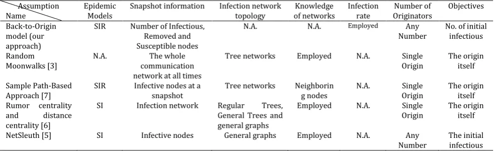
To achieve the above goals, we develop two models: deterministic Back-to-Origin model and stochastic Back-to-Origin Markov model for homogeneous random scanning worms. In stochastic Back-to-Origin model, we run time backwards. We assume to have the number of susceptible, infectious and removed nodes at a time snapshot. The time evolves in reverse order of worm propagation. To the best of our knowledge, we are the first to develop stochastic Back-to-Origin worm propagation model to estimate the number of origin infectious nodes. These models may further be used to identify the origin of worm propagation and to reconstruct worm propagation path probabilistically. This method is agnostic to algorithms that need the complete network flow or network topology. Table 1 gives a comparison of the assumptions in our model and the above mentioned methods.
As shown in Table 1, our method does not require any prior knowledge about network topology. Our approach requires less storage space and less limiting assumptions in comparison with other proposed approaches in [3], [6]-[8] as it doesn’t deploy network topology and network flows. Our method does not make any assumptions about the initial condition of nodes in forward model.
In this paper, we first develop a deterministic Back-to-Origin model. For this model, we define susceptibility rate. In this model, we determine the number of susceptible, infectious and removed nodes backwards in time. Second, we propose a stochastic Back-to-Origin Markov model. The Back-to-Origin process has Markov property, because the state of the system at past has no influence on the future, if present is specified. We assume to have the number of susceptible, infectious and removed nodes at an arbitrary snapshot of Back-to-Origin model. Here, we reformulate the above deterministic Back-to-Origin model based on the Continuous-Time-Markov-Chain and estimate the number of infectious nodes at each time of worm propagation backwards in time.
Experiments on our deterministic Back-to-Origin model indicated that infection rate and susceptibility rate are almost equal when the time difference is small. We reliably predict the correct number of infectious nodes at each time point with our stochastic Back-to-Origin Markov model.
2.
Related Works and Preliminaries
Computer worms probe vulnerable hosts by different target discovery techniques. Worms are classified by their target discovery techniques to two classes: scan-based worms and topology-based worms [9]. Scan-based worms employ two target discovery techniques: random-scanning and localized-scanning. In random-scanning, worms seek targets randomly or through an ordered block, i.e. uniform scanning, hit-list scanning and routable scanning. In localized scanning, worms compromise IP addresses that are closer. They are classified to local preference scanning and local preference sequential scanning.
Table 1. Our Stochastic Back-to-Origin Markov Model Assumption
Name Epidemic Models Snapshot information Infection network topology of networks Knowledge Infection rate Originators Number of Objectives Back-to-Origin
model (our approach)
SIR Number of Infectious, Removed and Susceptible nodes
N.A. N.A. Employed Any Number
No. of initial infectious
Random Moonwalks [3]
N.A. The whole communication network at all times
Tree networks Employed N.A. Single Origin
The origin itself
Sample Path-Based
Approach [7] SIR Infective nodes at a snapshot Tree networks Neighboring nodes N.A. Origin Single The origin itself Rumor centrality
and distance centrality [6]
SI Infection network Regular Trees, General Trees and general graphs
Employed N.A. Single Origin
The origin itself
NetSleuth [5] SI Infective nodes General graphs Employed N.A. Any
Number The initial infectious
The first complete mathematical model for the spread of infectious diseases was the deterministic general epidemic model, proposed by Kermack and Mckendrick [10]. In epidemiology study for internet worms, hosts have three states: Susceptible (denoted by S), Infectious (denoted by I), and Removed (denoted by R). A node is infected, if it is infectious or removed. This model is called SIR model [1], [11], as is defined by the following set of differential equations:
( ) ( ) ( ) ( ) ( ) ( ) ( ) ( ) ( ) dS t
I t S t dt
dI t
I t S t I t dt dR t I t dt (1)
is the infection rate. It is the proportion of <infectious, susceptible> pairs that change the state of susceptible nodes to infectious state [1]. In other words, one infectious node infects S t( )susceptible
nodes at each time step (
dt
), and the number of infective nodes increases as the proportion () of contacts between infective and susceptible nodes at each time point:
I t S t( ) ( ).3.
Deterministic Back-to-Origin Model
3.1.
The Model
rate B. In order to determine the number of final infectious nodes in this model, (these are initial infectious hosts in worm propagation model), prior knowledge of the number of initial infectious and removed nodes is necessary (these are final infectious and removed nodes in SIR model).
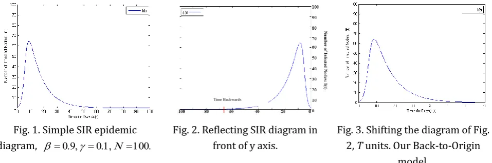
Fig. 1 shows the simulation of SIR epidemic model. In this model, time flows forward. Simulation parameters are as follows:
0.9,
0.1,N 100, whereN
is the total number of nodes.T
is the equilibrium time. The playing-time duration of the simulation is 100 seconds. Once the worm propagation reaches equilibrium for the first time, the number of susceptible, infectious and removed nodes doesn't change with time, dS dI dR 0dt dt dt .
Let us flip the diagram of Fig. 1 around its vertical axis (Fig. 2) and form a reflected diagram. Now we shift the reflected diagram (Fig. 2) horizontally, and add a constant to the time axis of it. This constant is time to equilibrium (In this example,
T
70
). The resulting diagram is our deterministic Back-to-Origin model, (Fig. 3), where
denotes the time running backwards in Back-to-Origin model and satisfies equation (2):,
t T
dt
d
(2)Consider
B and
B in Back-to-Origin model. We call
B a s susceptibility rate and
B as revive-ability rate.
B is the rate by which effective <infective, susceptible> pairs convert the infective to susceptible at each time unit. It is defined in equation (3).# of infectives that become susceptible by one susceptible infected space
B
(3)R
removed nodes become infectious with rate
B. At each time unit of our Back-to-Origin model,
B removed nodes become infectious. Comparing 1 and Fig. 3, it is interesting to note that the number of susceptible nodes contaminated at timet
in SIR diagram, is equal to the number of infectious nodes converted to susceptible at time in Back-to-Origin diagram, and we have the following simple equation (4).( )
( )
t T
dS t
dS
dt
d
(4)In SIR model, as the epidemic progresses in time
t
, theI
value increases and the value ofS
decreases, . In Back-to-Origin model, the progress of time
increases theS
value and decreases the value ofI
.In SIR epidemic model, each infective node contacts with susceptible nodes and these connections are selected with rate . In our Back-to-Origin model, we assume that each susceptible node contacts infective nodes and restores them to susceptible with rateB. Thus, BI t( ) infective nodes become
susceptible at each time by one susceptible node. Hence, the total number of susceptible nodes increases by the number of infective nodes that become susceptible, and
BI( ) ( )
S
counts the result of restoration by
( )
( ) ( )
( ) ( ) ( ) ( )
( )
B
B B
B
dS
S I
d dI
S I I
d dR
I d
(5)
dS dt
gives the slope of S t( ) at time
t
and dSdt
gives the slope of S( ) at time
. We consider timet
in SIR model and the corresponding time
in Back-to-Origin model. The slope of the curves in both models at corresponding times have equal absolute values. In this way, Back-to-Origin model is playing worm propagation model in reverse at corresponding times (t
and
).Fig. 1. Simple SIR epidemic diagram,
Fig. 2. Reflecting SIR diagram in front of y axis.
Fig. 3. Shifting the diagram of Fig. 2, T units. Our Back-to-Origin
model.
Given the equations (4) and (5), we describe the relationship betweenand Bas follows:
(1 ( ) )(1 ( ) )
B
t T
I t h S t h h
(6)
where
h
is close to zero. Ash
is very small, B is very close to , but it is a negative value.From equation (6), we conclude that B is dependent on time. Because
h
is close to zero,denominator of equation (6) is almost equal to one and thus B and are almost equal. Therefore
susceptibility rate and infection rate are very close values. This result is quite natural, since the rate at which susceptible hosts become infectious at each time unit is almost equal to the rate at which infectious nodes become susceptible at corresponding time of our Back-to-Origin model.
3.2.
Simulation
We ran simulation experiments for homogeneous random scanning worms and simulated the propagation of a random scanning worm in VC++. We chose different values for infection and removed rates in each experiment. Simulations were run for 800 seconds, and each second is divided to DIVIDE_SECOND units. Here, SIR model has been adopted and verified for the propagation of computer worms, and we are only playing the film backwards. Here we report on experimental investigations of worm propagation. A susceptible host became infectious only by contacting with an infectious host with rate (infection rate). Infectious host’s state turns to removed state with rate
(removal rate). We increased the number of initially infectious hosts from 1 to NUM (NUM is the number of initialsusceptible hosts). Parameters used for our experiments are shown in Table 2. Here, we try to give an example to show that our model is correct. We use a numerical simulation to assess the correctness of our model. We try only 50 nodes to demonstrate its correctness and to avoid unnecessary complications.
Counting the number of susceptible, infectious and removed nodes at each time step of worm propagation, we find differences between susceptible populations in two consecutive time steps. Let
S
denote the difference between the number of susceptible nodes. We used equations (7) and (8) to estimate and B.
( ) ( )
S t S t I t
(7)
( )
( ) ( )
B
S
S I
(8)
In this experiments, we used time steps
DIVIDE SECOND
1
t
. Comparing and B at different
time steps of each simulation run, shows that time steps with smaller
S
values, causes smaller differences betweenand B, because equation (5) holds when
t
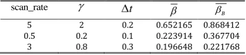
approaches 0. We show average valuesof and B in our experiments in Table 2. With higher scan rate values (i.e.
scan_rate=5
), the difference between
and B increases, because equation (6) holds when
t
approaches 0.Table 2. Parameter Values in Our Experiments
scan_rate
t
B
5 2 0.2 0.652165 0.868412
0.5 0.2 0.1 0.223914 0.367704
3 0.8 0.3 0.196648 0.221768
4.
Stochastic Back-to-Origin Markov Model
4.1.
The Model
Consider our deterministic Back-to-Origin worm model with parameters i s r, , ,
B, where s is thenumber of susceptible nodes,
i
is the number of infective nodes andr
is the number of removed nodes at current time. B is the susceptibility rate. Define stochastic processes I t( ) and R t( ), the number ofinfective and removed nodes at time
t
. The process ( , ) {( ( ), ( ));i r I t R t t 0} is a Markov process,because the state of the system at next time is only dependent on the current state of the system and not dependent on the previous state of the system. We consider Continuous-Time-Markov-Chain (CTMC) with the state ( ( ), ( ))I t R t ( , )i r . Then the transition rates at the state ( , )i r in Back-to-Origin Markov model can be described as follows:
A removed node becomes infectious, so the transition rate to the state (i1,r1) is given by:
,
i r B
i
(9)An infectious node can be vulnerable with rate B. The transition rate to the state (i1, )r is given by:
,
(
)
i r B
i N
i
r
The transition diagram is shown in Fig. 4.
Fig. 4. Transition diagram for Stochastic Back-to-Origin Markov model.
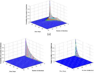
(a)
Fig. 5. Probability distribution of the number of infective nodes at time t, (a) Experiment 1, (b) Experiment 2, (c) Experiment 3.
Consider the probability,
,
Pr{ ( )
, ( )
}
i r
P
I t
i R t
r
,
( )
i r
P
t
is the probability thati
nodes are infectious andr
nodes are removed at timet
. Using Equations (9) , (10), we obtain the following difference-differential equation:(11) where,
i r,
i r,
i r, .,
( )
1, 1,( )
1, 1 1, 1( )
, ,( )
i r i r i r i r i r i r i r
d
P
t
P
t
P
t
P
t
Marginal distribution of
P
i r,( )
t
averaging overr
provides the probability distribution ofP t
i( )
, the probability thati
nodes are infectious at timet
.We calculated marginal distribution of
P
i r,( )
t
averaging overr
, applying equation (13)., ,
1, 1, 1
,
( ) ( )
( 1)( 1) ( ) ( 1) ( )
( ( )) ( )
i r i r
B i r B i r
B B i r
P t t P t
i N i r P t i P t
t
N i r iP t
(12)
, 1, 1 1
, ,
( ) ( ( 1)( 1) ( ) ( 1) ( ) ( ( )) ( )) ( )
i r B i r B i r
B B i r i r
P t t i N i r P t i P t
N i r iP t t P t
(13)
We provide a Matlab program to calculate differential equation (13) and marginal probability distribution of
( )
i
P t
as a function of time at time step
t
. For illustrative purposes, we chose different parameter values fori r
, ,
B,
B,
t
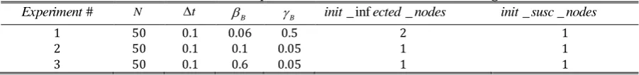
. Table 3 lists the model parameters and their initial values. The plots (see Fig. 5) show the probability of the number of infective nodes at each time point.Table 3. Parameter Values in Our Experiments for Stochastic Back-to-Origin Markov Model
#
Experiment N t B B init_ infected_nodes init_susc nodes_
1 50 0.1 0.06 0.5 2 1
2 50 0.1 0.1 0.05 1 1
3 50 0.1 0.6 0.05 1 1
5.
Concluding Remarks and Future Works
In this paper, we studied predicting the number of infectious nodes, at different time of spreading a homogeneous random scanning worm. We developed two models: deterministic Back-to-Origin model and stochastic Back-to-Origin Markov model. Assuming the SIR model and using a snapshot in which we know the number of susceptible, infectious and removed nodes, we derive probability distributions to estimate the number of infectious nodes. These models help in quantifying the relationship between worm infection rate, the final size of epidemic and initial size of the infected population based on probability. To our knowledge, our Back-to-Origin models are the first of their kind presented in open literature. Compared with other methods that identify the origin or the number of initial nodes, our method requires to store less information about nodes and network and has less limiting assumptions. Other mentioned methods need to store network topology or network flows. Our method needs a snapshot in which we know the number of infectious and removed nodes and it needs to know the infection and removed parameters.
We demonstrated through simulations that these models can be highly effective in estimating the size of worm origins. Experiment and analysis show that infection rate and susceptibility rate are almost equal parameters. Experiments show that our stochastic model predict the number of infectious nodes. These models does not need any prior knowledge about network topology. An open problem is how to identify the origin of worm propagation and to reconstruct worm propagation path with the help of the derived probability distribution, while assuming some practically collectable data.
References
[1] Daley,D. J., & Gani, J. (2001). Epidemic Modeling: An Introduction, Cambridge University Press.
moonwalks. Proceedings of IEEE Symposium on Security and Privacy.
[3] Zhu, K., & Ying, L. (2014). Information source detection in the SIR model: A sample path based approach, IEEE/ACM Transactions on Networking, 1, 99.
[4] Shah, D., & Zaman, T. (2010). Detecting sources of computer viruses in networks: theory and experiment, ACM SIGMETRICS International Conference on Measurement and Modeling of Computer Systems (pp. 203-214). New York.
[5] Prakash, B. A., Vrekeen, J., & Faloutsos, C. (2012). Spotting culprits in epidemics: How many and which ones. Proceedings of IEEE 12thinternational Conference in Data Mining (pp. 11-20). Washington, DC.
[6] Chen, Z., Gao, L., & Kwiat, K. (2003, March) Modeling the spread of active worms. Proceedings of the IEEE Conference on Computer Communications (INFOCOM), (pp. 1890-1900), SN Francisco, CA.
[7] Chen, Z., Zhu, K., & Ying L., (2014). Detecting multiple information sources in networks under the SIR model. Proceedings of the 48thConference on Information Sciences and Systems, (pp. 1-4). Princeton, NJ.
[8] Okamura, H., Kobayashi, H., & Dohi, T. (2005). Markovian modeling and analysis of internet worm propagation. Proceedings of 16th IEEE International Symposium on Software Reliability Engineering (pp. 149-158). Chicago, IL.
[9] Wang, Y., Wen, S., Xiang, Y., & Zhou, W. (2014). Modeling the propagation of worms in networks: A survey. IEEE Communication Surveys and Tutorials, 16(2), 942-960.
[10]M. J., Kermack, & McKendrick, A. G. (1927). A Contribution to the mathematical theory of epidemics. Bulletin of Mathematical Biology, 53(1-2), 89-118.
[11]Xiang, Y., Fan, X., & Zhu, W. T. (2009). Propagation of active worms: A survey. International Journal of Computer Systems Science and Engineering, 24(2), 157-172.
Tala Tafazzoli was born in Tehran, Iran, in 1974. She received the B.S. degree from Sharif University of Technology, Tehran, Iran, in 1995 and M.S. degree from Amirkabir University of Technology, Tehran, in 1997, both in computer engineering. She is currently pursuing the Ph.D. degree with the Department of Computer and IT Engineering, Amirkabir University of Technology. She is also a faculty member of Research Institute of ICT. Her research interests include digital forensics, malware forensics and information security.