Particle Swarm Optimization Algorithm for the
Shortest Confidence Interval Problem
Shang Gao and Zaiyue Zhang
School of Computer Science and Engineering, Jiangsu University of Science and Technology, Zhenjiang 212003, China
Email: [email protected] [email protected]
Cungen Cao
Institute of Computing Technology,The Chinese Academy of Sciences,Beijing 100080, China Email: [email protected]
Abstract—Based on the example of constructing a
confidence interval for variance, the notion and construction of the shortest confidence interval are put forward. Furthermore, the particle swarm algorithm for this problem is presented to solve this non-linear programming problem. Compared with the confidence interval calculated with traditional method, it has distinct advantage. The optimum results which is used to find the shortest confidence interval of variance and mean variance are given under the confidence level 0.9 and 0.95. The shortest confidence interval about Gamma distribution, Laplace distribution, Weibull distribution and beta distribution are also discussed.
Index Terms—mathematical statistics, confidence interval,
the shortest interval, particle swarm algorithm
I. INTRODUCTION
The confidence interval of unknown parameter represents the range of the value and the reliability about estimation of parameter. Under given confidence level,the length of confidence interval represents the precision of the estimation. It is very necessary to research the problem how to construct good random variables to make the length of confidence interval as short as possible. In practical applications,People generally get confidence interval by probability symmetry. But the length of this kind of confidence interval is not the shortest. Although most introductory textbooks in mathematical statistics discuss confidence intervals, the concept of a shortest confidence interval commands little or no attention. Ramachandran (1958) and Tate and Klett (1959) specify shortest unbiased confidence intervals for the variance of a normal distribution. In addition, Ramachandran (1958) specifies the shortest unbiased confidence intervals for the ratio of two normal variances. Tate and Klett (1959) and Guenther (1969) also specify the physically shortest intervals for the variance of a single normal distribution.
The method of obtaining such an interval of binomial probability is presented as well by Zielinski Wojciech (2010). K.K. Ferentinos (2006) clarify and comment on methods of finding such intervals, investigate the relationship between these types of intervals, point out that confidence intervals with the shortest length do not always exist, even when the distribution of the pivotal quantity is symmetric; and finally, and give similar results when the Bayesian approach is used. In this paper
the shortest confidence interval about
2 and
of normal distribution are given under the confidence level 0.90 and 0.95. Finally, this paper gives the condition that the shortest confidence interval about Gamma distribution, Laplace distribution, Weibull distribution and Beta distribution.II. THE SHORTEST CONFIDENCE INTERVAL
A. The Shortest Confidence Interval
Let
X
1,
X
2,
,
X
n be a random sample from a distribution with probability density functionf
(
x
;
)
. In using the standard method for obtaining a confidence interval for
, one seeks a random variable)
(
)
;
,
,
,
(
X
1X
2X
T
T
n
whose distribution isindependent of
. Then the probability statement
a
T
(
)
b
1
P
is converted to
P
W
1
W
2
1
and, after observing
x
1,
x
2,
,
x
n, the specific numbers2 1
,
w
w
are calculated and form the endpoints of the confidence interval. For everyT
(
)
,a
andb
can be chosen in different ways, one of which is makew
2
w
1a minimum[5]. Such an interval is the shortest interval based upon
T
(
)
.Supported by National Basic Research Program of Jiangsu Province University (08KJB520003).
B. Shortest Confidence Interval of
2 of Normal DistributionSuppose
X
1,
X
2,
,
X
n are independent and identically distributed (iid) observations of a normalsample, say
N
(
,
2)
. Then,2 2
)
1
(
S
n
~
2(
n
1
)
Thus, we have
(
1
)
1
)
1
(
)
1
(
2 22 2
1 2 2
n
S
n
n
P
(1)which gives the
1
level confidence interval for
2 as
(
1
)
)
1
(
,
)
1
(
)
1
(
2 1 2 2 2 2 2n
S
n
n
S
n
(2)Obviously, the interval (2) can not guarantee the shortest length confidence interval. The following illustrate the concept and the method to find the shortest confidence interval.
(
1
)
1
)
1
(
)
1
(
2 22 2 ) ( 1
n
S
n
n
P
Then
1
)
1
(
)
1
(
)
1
(
)
1
(
2 ) ( 1 2 2 2 2n
S
n
n
S
n
P
The confidence interval is
(
1
)
)
1
(
,
)
1
(
)
1
(
2 ) ( 1 2 2 2n
S
n
n
S
n
(3)With length 2 2 2 ) ( 1 2 2 2 ) ( 1 2
)
1
](
)
1
(
1
)
1
(
1
[
)
1
(
)
1
(
)
1
(
)
1
(
2S
n
n
n
n
S
n
n
S
n
L
The problem of the shortest confidence interval problem is to find some suitable
which minimize2
'
L
.)
1
(
1
)
1
(
1
'
min
2 2) ( 1 2
n
n
L
(4)Programming (4) is an unconstrained non-linear programming problem about
. The objective function contains percentile, so it is hard to solve by derivative methods. In general, we can use direct search optimization methods, such as "random method", "random direct method" , "simplex method", etc.. In this paper, we use particle swarm optimization to solve thisproblem. The
2*(
n
)
is calculated by Matlab statisticstoolbox. X= chi2inv(P,V) computes the inverse of the
2
cumulative distribution function with parameters specified by V for the corresponding probabilities in P. P and V can be vectors, matrices, or multidimensional arrays that have the same size. A scalar input is expanded to a constant array with the same dimensions as the other inputs.III. THE PARTICLE SWARM OPTIMIZATION ALGORITHM
A. BasicPparticle Swarm Optimization (PSO) Algorithm In the particle swarm optimization (PSO) algorithm[7-9], the birds in a flock are symbolically represented as particles. These particles can be considered as simple agents “flying” through a problem space. A particle’s location in the multi-dimensional problem space represents one solution for the problem. When a particle moves to a new location, a different problem solution is generated. This solution is evaluated by a fitness function that provides a quantitative value of the solution’s utility.
The velocity and direction of each particle moving along each dimension of the problem space will be altered with each generation of movement. In combination, the particle’s personal experience, Pid and
its neighbors’ experience, Pgdinfluence the movement of
each particle through a problem space. The random values rand1 and rand2 are used for the sake of
completeness, that is, to make sure that particles explore a wide search space before converging around the optimal solution. The values of c1 and c2 control the weight
balance of Pid and Pgd in deciding the particle’s next
movement velocity. At every generation, the particle’s new location is computed by adding the particle’s current velocity, vid, to its location, xid. Mathematically, given a multi-dimensional problem space, the ith particle changes its velocity and location according to the following equations[7-9]:
)
(
)
(
2 2 1 1 0 id gd id id id idx
p
rand
c
x
p
rand
c
v
c
v
(5) id id idx
v
x
(6) where c0 denotes the inertia weight factor; pid is thelocation of the particle that experiences the best fitness value; Pgdis the location of the particles that experience a
global best fitness value; c1 and c2 are constants and are
known as acceleration coefficients; d denotes the dimension of the problem space; rand1, rand2are random
values in the range of (0, 1). For equation (1), the first part represents the inertia of pervious velocity; the second part is the “cognition” part, which represents the private thinking by itself; the third part is the “social” part, which represents the cooperation among the particles. If the sum of accelerations would cause the velocity vid, on that
dimension to exceed vmax,d ,then vid, is limited to vmax,d.
vmax,d determines the resolution with which regions
B. PSO Algorithm For The Shortet Confidence Interval Problem
The PSO algorithm for the shortest confidence interval problem can be described as follows:
I) Initialize particle
a) Set constants c0, c1and c2..
b) Randomly initialize particle positions. c) Randomly initialize particle velocities. II) Do:
a) For each particle:
1) Calculate fitness value (the
L
'
2).2) If the fitness value is better than the best fitness value Pid in history.
3) Set current value as the new Pid.
End
b) For each particle:
1) Find in the particle neighborhood, the particle with the best fitness Pgd.
2) Calculate particle velocity according to the velocity equation (5).
3) Apply the velocity constriction.
4) Update particle position according to the position equation (6).
5) Apply the position constriction. End
While maximum iterations or minimum error criteria is not attained.
C.Rresults
According to this algorithm using Matlab language, the values of
*
at which is used to find the shortest confidence interval of
2 with
0
.
1
and
0
.
05
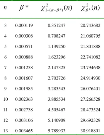
are shown in table1 and table 2.TABLE I.
THE VALUES OF
*
WHICH IS USED TO FIND THE SHORTEST CONFIDENCE INTERVAL OF
2 WITH
0
.
1
n
*
12(*)(
n
)
2*(
n
)
3 0.000522 0.5820809 17.639246 4 0.001176 1.0560833 18.107127 5 0.001999 1.593792 18.908544 6 0.002916 2.175047 19.874058 7 0.003875 2.788257 20.930096 8 0.004841 3.426202 22.040714 9 0.005795 4.084034 23.184494 10 0.006724 4.758364 24.349852 11 0.007621 5.446704 25.529312 12 0.008482 6.147173 26.718172 13 0.009307 6.858268 27.912678
14 0.010095 7.578826 29.110953 15 0.010847 8.307880 30.311355 16 0.011565 9.044611 31.512560 17 0.012250 9.788358 32.713942 18 0.012904 10.538536 33.914829 19 0.013529 11.294641 35.114730 20 0.014125 12.056287 36.313788 21 0.014696 12.823028 37.511158 22 0.015243 13.594543 38.706840 23 0.015766 14.370579 39.901094 24 0.016268 15.150817 41.093440 25 0.016749 15.935059 42.284150 26 0.017212 16.723027 43.472766 27 0.017657 17.514560 44.659550 28 0.018084 18.309517 45.844744 29 0.018496 19.107657 47.027886 30 0.018893 19.908863 48.209203 31 0.019276 20.712987 49.388682 32 0.019645 21.519932 50.566525 33 0.020002 22.329526 51.742473 34 0.020347 23.141686 52.916709 35 0.020681 23.956291 54.089182
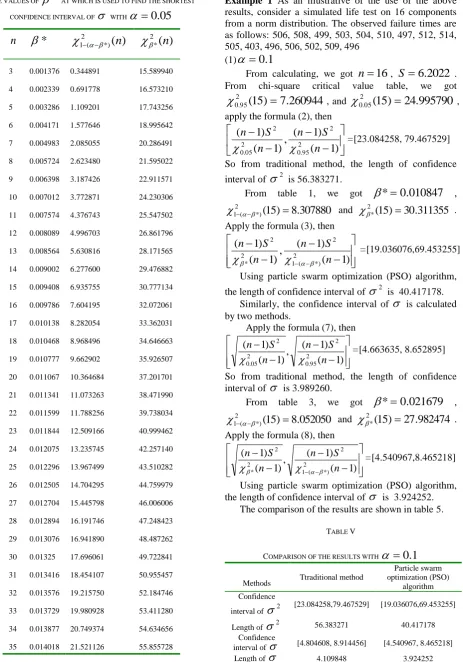
TABLE II
THE VALUES OF
*
WHICH IS USED TO FIND THE SHORTEST CONFIDENCE INTERVAL OF
2 WITH
0
.
05
n
*
12(*)(
n
)
2*(
n
)
14 0.003814 6.450983 32.149934 15 0.004152 7.122802 33.384027 16 0.004479 7.804332 34.619444 17 0.004794 8.494722 35.855844 18 0.005098 9.193190 37.091861 19 0.005391 9.899099 38.327132 20 0.005674 10.611859 39.560851 21 0.005946 11.331038 40.793575 22 0.006209 12.056132 42.024135 23 0.006462 12.786820 43.253213 24 0.006706 13.522734 44.480358 25 0.006942 14.263534 45.705179 26 0.007170 15.008963 46.927861 27 0.007390 15.758788 48.148585 28 0.007602 16.512804 49.367528 29 0.007808 17.270706 50.583838 30 0.008006 18.032442 51.798728 31 0.008199 18.797672 53.010855 32 0.008385 19.566376 54.221404 33 0.008566 20.338296 55.429552 34 0.008741 21.113374 56.635956 35 0.008911 21.891432 57.840285
IV.SHORTEST CONFIDENCE INTERVAL OF
The confidence interval for
is
(
1
)
)
1
(
,
)
1
(
)
1
(
2 1
2 2
2
2 2
n
S
n
n
S
n
(7)The length of
isS
n
n
n
n
S
n
n
S
n
L
1
]
)
1
(
1
)
1
(
1
[
)
1
(
)
1
(
)
1
(
)
1
(
2 2
) ( 1
2 2 2
) ( 1
2
(8)
The problem of the shortest confidence interval
problem is to find some suitable
which minimizeL
'
.)
1
(
1
)
1
(
1
'
min
2 2
) (
1
n
n
L
(9)Use the above method recount, the values of
*
at which is used to find the shortest confidence interval of
with
0
.
1
and
0
.
05
are shown in table3 and table 4.TABLE III.
THE VALUES OF
*
AT WHICH IS USED TO FIND THE SHORTEST CONFIDENCE INTERVAL OF
WITH
0
.
1
n
*
12(*)(
n
)
2*(
n
)
TABLE IV.
THE VALUES OF
*
AT WHICH IS USED TO FIND THE SHORTEST CONFIDENCE INTERVAL OF
WITH
0
.
05
n
*
12(*)(
n
)
2*(
n
)
3 0.001376 0.344891 15.589940 4 0.002339 0.691778 16.573210 5 0.003286 1.109201 17.743256 6 0.004171 1.577646 18.995642 7 0.004983 2.085055 20.286491 8 0.005724 2.623480 21.595022 9 0.006398 3.187426 22.911571 10 0.007012 3.772871 24.230306 11 0.007574 4.376743 25.547502 12 0.008089 4.996703 26.861796 13 0.008564 5.630816 28.171565 14 0.009002 6.277600 29.476882 15 0.009408 6.935755 30.777134 16 0.009786 7.604195 32.072061 17 0.010138 8.282054 33.362031 18 0.010468 8.968496 34.646663 19 0.010777 9.662902 35.926507 20 0.011067 10.364684 37.201701 21 0.011341 11.073263 38.471990 22 0.011599 11.788256 39.738034 23 0.011844 12.509166 40.999462 24 0.012075 13.235745 42.257140 25 0.012296 13.967499 43.510282 26 0.012505 14.704295 44.759979 27 0.012704 15.445798 46.006006 28 0.012894 16.191746 47.248423 29 0.013076 16.941890 48.487262 30 0.01325 17.696061 49.722841 31 0.013416 18.454107 50.955457 32 0.013576 19.215750 52.184746 33 0.013729 19.980928 53.411280 34 0.013877 20.749374 54.634656 35 0.014018 21.521126 55.855728
V. NUMERICAL EXAMPLES
Example 1 As an illustrative of the use of the above results, consider a simulated life test on 16 components from a norm distribution. The observed failure times are as follows: 506, 508, 499, 503, 504, 510, 497, 512, 514, 505, 403, 496, 506, 502, 509, 496
(1)
0
.
1
From calculating, we got
n
16
,S
6
.
2022
. From chi-square critical value table, we got260944
.
7
)
15
(
295 .
0
, and
02.05(
15
)
24.995790
,apply the formula (2), then
)
1
(
)
1
(
,
)
1
(
)
1
(
2 95 . 0
2
2 05 . 0
2
n
S
n
n
S
n
=[23.084258, 79.467529]So from traditional method, the length of confidence
interval of
2 is 56.383271.From table 1, we got
*
0
.
010847
,307880
.
8
)
15
(
2*) (
1
and
2*(
15
)
30
.
311355
.Apply the formula (3), then
(
1
)
)
1
(
,
)
1
(
)
1
(
2 *) ( 1
2
2 *
2
n
S
n
n
S
n
=[19.036076,69.453255]Using particle swarm optimization (PSO) algorithm,
the length of confidence interval of
2 is 40.417178. Similarly, the confidence interval of
is calculated by two methods.Apply the formula (7), then
)
1
(
)
1
(
,
)
1
(
)
1
(
2 95 . 0
2
2 05 . 0
2
n
S
n
n
S
n
=[4.663635, 8.652895]So from traditional method, the length of confidence interval of
is 3.989260.From table 3, we got
*
0
.
021679
,052050
.
8
)
15
(
2*) (
1
and
2*(
15
)
27
.
982474
.Apply the formula (8), then
( 1)
) 1 ( , ) 1 (
) 1 (
2 *) ( 1
2
2 *
2
n S n n
S n
=[4.540967,8.465218]Using particle swarm optimization (PSO) algorithm, the length of confidence interval of
is 3.924252.The comparison of the results are shown in table 5.
TABLE V
COMPARISON OF THE RESULTS WITH
0
.
1
Methods Ttraditional method
Particle swarm optimization (PSO)
algorithm Confidence
interval of
2 [23.084258,79.467529] [19.036076,69.453255] Length of
2 56.383271 40.417178Confidence
(2)
0
.
05
From chi-square critical value table, we got
262138
.
6
)
15
(
2 975 . 0
and 2(
15
)
2
7.488393
025 .
0
,apply the formula (2), then
)
1
(
)
1
(
,
)
1
(
)
1
(
2 975 . 0 2 2 025 . 0 2n
S
n
n
S
n
=[20.991015, 92.14258]So from traditional method, the length of confidence
interval of
2 is 71.151523.From table 2, we got
*
0
.
004152
,122802
.
7
)
15
(
2 *) (1
and
2*(
15
)
33
.
384027
.Apply the formula (3), then
(
1
)
)
1
(
,
)
1
(
)
1
(
2 *) ( 1 2 2 * 2n
S
n
n
S
n
=[17.283993,81.008748]Using particle swarm optimization (PSO) algorithm,
the length of confidence interval of
2 is 63.724756. Similarly, the confidence interval of
is calculated by two methods.Apply the formula (7), then
)
1
(
)
1
(
,
)
1
(
)
1
(
2 975 . 0 2 2 025 . 0 2n
S
n
n
S
n
=[4.581595, 9.599091]So from traditional method, the length of confidence interval of
is 5.017495.From table 4, we got
*
0
.
009408
,935755
.
6
)
15
(
2 *) (1
and
2*(
15
)
30
.
777134
.Apply the formula (8), then
(
1
)
)
1
(
,
)
1
(
)
1
(
2 *) ( 1 2 2 * 2n
S
n
n
S
n
=[4.329894, 8.317557]Using particle swarm optimization (PSO) algorithm, the length of confidence interval of
is 3.987663.The comparison of the results are shown in table 6.
TABLE VI
COMPARISON OF THE RESULTS WITH
0
.
05
Methods Ttraditional method
Particle swarm optimization (PSO)
algorithm Confidence
interval of
2 [20.991015, 92.14258][17.283993,81.008748]
Length of
2 71.151523 63.724756. Confidenceinterval of
[4.581595, 9.599091] [4.329894, 8.317557] Length of
5.017495 3.987663VI. DISCUSSION
A. The Shortest Confidence Interval For Gamma Distributions
Above all, the minimum length of confidence interval for the variance of the normal distribution are discussed.
In fact, the shortest confidence interval for other distributions can use the results of table1.
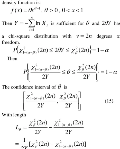
Let
X
have a gamma distribution with parameters
and
and assume that
is a known integer. Thus, the density function ofX
is
xe
x
T
x
f
1 )
(
1
)
(
A sufficient statistic for
is
n i iX
Y
1and
2
Y
has a chi-square distribution with
v
2
n
degrees of freedom.
(
2
)
1
2
)
2
(
2 2 ) ( 1n
Y
n
P
Then
1
)
2
(
2
)
2
(
2
2 ) ( 1 2n
Y
n
Y
P
The confidence interval of
is
(
2
)
2
,
)
2
(
2
2 ) ( 12
n
Y
n
Y
(10) With length]
)
2
(
1
)
2
(
1
[
2
2 2) (
1
n
n
Y
L
The problem of the shortest confidence interval problem
is to find some suitable
which minimizeL
'
.)
2
(
1
)
2
(
1
'
min
2 2) (
1
n
n
L
(11)
Thus the solution for
12(*)(
n
)
and
2*(
n
)
isthe same as table 1 with
0
.
1
or the same as table 2 with
0
.
05
.B. The Shortest Confidence Interval For Laplace Distributions
Let
X
have the Laplace distribution with probability density function
x
e
x
f
2
1
)
(
,
0
Then
n i iX
Y
1is a sufficient statistic for
and
Y
2
has a chi-square distribution withv
2
n
degreesof freedom.
(
2
)
1
Then
1
)
2
(
2
)
2
(
2
2 ) ( 1 2
n
Y
n
Y
P
The confidence interval of
is
(
2
)
2
,
)
2
(
2
2 ) ( 1 2
n
Y
n
Y
(12)With length
]
)
2
(
1
)
2
(
1
[
2
2 2) (
1
n
n
Y
L
The problem of the shortest confidence interval problem
is to find some suitable
which minimizeL
'
.)
2
(
1
)
2
(
1
'
min
2 2) (
1
n
n
L
(13)
Thus the solution for
12(*)(
n
)
and
2*(
n
)
is also the same as table 1 with
0
.
1
or the same as table 2 with
0
.
05
.C. The Shortest Confidence Interval For Weibull Distributions
Let
X
have the Weibull distribution with probability density function
xe
x
x
f
(
)
1 ,
0
,x
0
With
0
being known. Then
n ii
X
Y
1
is a
sufficient statistic for
and2
Y
has a chi-squaredistribution with
v
2
n
degrees of freedom as in Example 3. when
1
, it is exponential distribution. The probability density function is
xe
x
f
(
)
1
,
0
,x
0
(14)This conclusion include the shortest confidence interval for exponential distribution.
D. The Shortest Confidence Interval For Beta Distributions
The probability density function of the beta distribution is:
1 1
)
1
(
)
(
)
(
)
(
)
(
x
x
x
f
,
0
,0
x
1
where
is the gamma function.The beta density function can take on different shapes depending on the values of the two parameters. Here, we
discuss beta distribution with
1
. The probability density function is:1
)
(
x
x
f
,
0
,0
x
1
Then
ni
i
X
Y
1
ln
is sufficient for
and2
Y
hasa chi-square distribution with
v
2
n
degrees of freedom.
12()(
2
n
)
2
Y
2(
2
n
)
1
P
Then
1
2
)
2
(
2
)
2
(
22 ) ( 1
Y
n
Y
n
P
The confidence interval of
is
Y
n
Y
n
2
)
2
(
,
2
)
2
(
22 ) (
1
(15)
With length
)]
2
(
)
2
(
[
2
1
2
)
2
(
2
)
2
(
2 ) ( 1 2
2 ) ( 1 2
n
n
Y
Y
n
Y
n
L
The problem of the shortest confidence interval problem
is to find some suitable
which minimizeL
'
.)
2
(
)
2
(
'
min
L
2n
12()n
(16) According to this algorithm using Matlab language, the values of
*
at which is used to find the shortest confidence interval of
with
0
.
1
is shown in table 6.TABLE VI
THE VALUES OF
*
WHICH IS USED TO FIND THE SHORTEST CONFIDENCE INTERVAL OF
WITH
0
.
1
n
*
12(*)(
n
)
2*(
n
)
26 0.069176 14.276393 37.371892 28 0.068473 15.815528 39.829571 30 0.067841 17.371860 42.270631 32 0.067270 18.943504 44.696663 34 0.066751 20.528957 47.109084 36 0.066275 22.127091 49.509245 38 0.065838 23.736672 51.898039 40 0.065434 25.356855 54.276463 42 0.065060 26.986736 56.645219 44 0.064712 28.625651 59.005053 46 0.064386 30.273071 61.356687 48 0.064081 31.928305 63.700538 50 0.063795 33.590841 66.037085 52 0.063526 35.260245 68.366787 54 0.063272 36.936151 70.690081 56 0.063031 38.618256 73.007394 58 0.062803 40.306107 75.318934 60 0.062587 41.999388 77.624991 62 0.062381 43.697933 79.925951 64 0.062186 45.401288 82.221869 66 0.061999 47.109460 84.513220 68 0.061820 48.822162 86.800149 70 0.061649 50.539125 89.082787
VII. CONCLUSIONS
The interval estimation of parameter is a basic form for statistical conclusion, which can indicate the possible scale for estimated general parameter in a certain extent dependability based on the distribution of pivot quantity. The theory of Neyman confidence interval shows that the certain level of confidence ensures the certain extent dependability, but the precision is often scaled by the length of interva1. The shortest confidence interval problem is a non-linear programming problem and the particle swarm algorithm for this problem is presented to solve it. The optimum results which is used to find the
shortest confidence interval of
2 and
are given under the sample sizes from 4 to 36 and the confidence level 0.9. The shortest confidence interval about Gamma distribution, Laplace distribution and Weibull distribution can use results also. The results of the shortest confidence interval about Beta distribution are given also. When sample size is not large, conclusion shows that the precision of the interval estimation of parameter is remarkably increasing if the data from Tables in thispaper are used. The shortest confidence interval of other distribution can be obtained by similar method.
ACKNOWLEDGMENT
This work was partially supported by National Basic Research Program of Jiangsu Province University (08KJB520003) and the Open Project Program of the State Key Lab of CAD&CG.
REFERENCES
[1] W.C. Guenther, “Shortest confidence intervals”. The American Statistician , vol.23, no.1, pp.22-25,1969. [2] K.V. Ramachandran, “A test of variances”. Journal of the
American Statistical Association, vol.53, pp.741-747, 1958. [3] R.F. Tate and G.W. Klett , “Optimal confidence intervals
forth variance of a normal distribution”. Journal of the American Statistical Association, vol.54, pp.674-682,1959. [4] Zielinski, Wojciech, “The shortest Clopper-Pearson confidence interval for binomial probability”. Communications in Statistics: Simulation and Computation, vol.39, no.1, pp.188-193, January 2010.
[5] K.K. Ferentinos and K.X. Karakostas, “More on shortest and equal tails confidence intervals”. Communications in Statistics - Theory and Methods, vol.35, no.5, pp.821-829, 2006.
[6] J. Goodman, “On the definition of the 'best' confidence interval”. Reliability engineering, vol.7, no.4, pp.213-228, 1984.
[7] R. C. Eberhart and J. Kennedy. “A New Optimizer Using Particles Swarm Theory”. Proc. 6th International Symposium on Micro Machine and Human Science, Nagoya, Japan, 1995, pp. 39-43.
[8] Y. H. Shi and R. C. Eberhart. “A Modified Particle Swarm Optimizer”. IEEE International Conference on Evolutionary Computation, Anchorage, Alaska, May 4-9, 1998, pp.69-73.
[9] S. Gao and J. Y. Yang, Swarm Intelligence Algorithm and Applications. Beijing: China Water Power Press, 2006, pp.7-10(in Chinese).
Shang Gao was born in 1972, and received his M.S. degree in 1996 and Ph.D degree in 2006. He now works in school of computer science and technology, Jiangsu University of Science and Technology. He is an associate professor and He is engage mainly in systems engineering.
Zaiyue Zhang was born in 1961, and received his M.S. degree in mathematics in 1991 from the Department of Mathematics, Yangzhou Teaching College, and the Ph.D. degree in mathematics in 1995 from the Institute of Software, the Chinese Academy of Sciences. Now he is a professor of Jiangsu University of Science and Technology. His current research areas are recursion theory, knowledge representation and knowledge reasoning.