ISSN (e): 2250-3021, ISSN (p): 2278-8719 Vol. 06, Issue 05 (May. 2016), ||V3|| PP 26-31
Influential Factors Analysis of Full Waveform Inversion In Time
Domain For Near-Surface Velocity Modeling
Zhou Tiejun
1Fan Xingcai
2(1. Northeast Petroleum University, Daqing 163318, China; 2. Exploration and Development
Research Institute of Daqing Oilfield Co. Ltd. , Daqing 163712, China)
Abstract: Seismic wave velocity is one of the most important parameters in the process of seismic data processing and interpretation, which is significant for calculating the near-surface statics, migration, predicting rock parameters and reservoir inversion. The full waveform inversion(FWI) is recognized widely as a kind of high precision, multi-parameter inversion tool, so it plays an unique advantages role in the velocity modeling. Based on the full waveform inversion of the acoustic wave equation in time domain, try out the influential factors for velocity inversion on forward modeling, folds, dominant frequency of wavelet, array length and uniformity. Comprehensively analyze the influencing factors and to determine the optimal experience parameters. Use the FWI to establish the complex near-surface geological model, which is proved to be correct and practical in shallow.
Key: velocity modeling, FWI, conjugate gradient method, influential factors
I.
INTRODUCTION
With the exploration and development of the oilfield, at present the entire oil and gas exploration targets have focused on deeper and more complicated peripheral area, Also puts forward a higher request to the high precision velocity modeling and precise imaging, extraction and analysis of inversion parameters, comprehensive seismic geologic interpretation. Therefore an advanced geophysical technology is needed to develop imminently, especially the accurate inversion method[1]. Accurate velocity modeling is the premise of all high precision seismic exploration technologies which include imaging, inversion and interpretation. The accuracy of velocity directly affect not only the static correction and velocity analysis of seismic data but also the final imaging result for the complex near-surface structure area. It is very difficult for the conventional velocity analysis method to detect low-velocity interlayer and complex near-surface geologic model.
FWI based on the theory of wave equation can accurately describe the near-surface model, Which can overcome the problem of deflection in ray tracing and multiple reflections. So it can reveal the structural details and lithological changes for complex geological conditions. The theory of FWI was primarily introduced in the 1980s. Both Lailly[2] and Tarantola[3] come up with FWI in time domain that transfers the problem of seismic exploration into a local optimization, which laid the theoretical foundation of FWI. Because of the wavefield can also propagation in frequency domain, Pratt[4] extended FWI to frequency-space domain in the 1990s. Frequency domain inversion can work out several preponderant frequencies individually, since the wavefield can be solved directly in the frequency domain. So it is easy to implement multi-scale inversion from low frequency to high frequency[5]. Because of the importance of low frequency, FWI in Laplace domain was came up with by Shin[6-7], which aims at taking advantage of the non-sensitivity to restore the low frequency data in the Laplace domain[8]. Of course FWI also produced many mixed inversions in the process of development. Such as hybrid domain inversion which combines propagation in time domain with inversion in frequency domain, Laplace domain combined with frequency domain, etc[9]. For all kinds of FWI, everyone of time domain, frequency domain, the Laplace domain or mixed domain has its usage, advantages and disadvantages.
Based on the full waveform inversion of the acoustic wave equation in time domain, analyze the influential factors for velocity inversion on forward modeling, folds, dominant frequency of wavelet, array length and uniformity. Comprehensively analyze the influencing factors, and to determine the optimal experience parameters. According to the trial of complex near-surface geological model, which is proved to be correct and practical in shallow complex near-surface velocity modeling accurately.
Principle of FWI in time domain
FWI minimizes the error between the waveform curve obtained by propagation forward of velocity model and observed in surface. Make the initial velocity model iteratively converge along the gradient. Therefor
1 Author introduction: Zhou Tiejun(1990-), male, master graduate student, majored in seismic processing and research.
Email:[email protected] Fund project:Supported by Northeast Petroleum University Innovation Foudation For
rebuild the real underground velocity model.
Acoustic wave equation of constant density can be expressed
s s s
s x t x f x t x u t x t x u x v ; , ; , ; , 1 2 2 2
2
(1)
Where 2 2 2 2 2 z x
, f
x,t;xs
is the wavelet in the shot-points.Besides, define a residual vector u ucal uobs , where uobs is the actual data observed from surface detectors, and ucal is the mimetic data calculated by velocity model. In the sense of least squares, the misfit function is
ng r ns s t s r obs s r cal T x t x u x t x u dt u u u u v E1 1 0
2 * max ; , ; , 2 1 2 1 2 1
(2)
Where ns and ng respectively represent the number of sources and geophones. u And u* respectively represent adjoint matrix and complex conjugate matrix of residual vector u .
Within the framework of Born approximation theory, N-dimensional velocity v can be expressed as the sum of initial velocity model v0 and the disturbance velocity v , namely v v0 v.Substituting it into the differentiation of equation (2) gives
v E H v v E v v E
v
1 0 1 2 0 2
(3)
Where Ev is the gradient vector, H 1 is the inverse matrix of Hessian. Based on conjugate gradient theory, we can get the update formula of velocities
k k k
k v g
v 1 (4) In the iterative process of gradient gk, the misfit function continuously converges in the direction of the gradient.
ux t x x x tdx dt
v t x t x u v v E v g ng r ns s V r s r s cal t i 1 1 * 3 2 2 0 , ; 0 , * ; , 2 ; , Re max
(5)
According to the conjugate state method of PLessix[10], that is to say, the conjugate state method is a way of reversing backward propagation the residual error by the conjugate of forward operator.
We have the following definition for conjugate gradient
0 0
1, g
gk k k
k
(6) Where k is the iterative correction factor of conjugate gradient. In order to get faster convergence rate, we use a hybrid factor based on the method of Hesteness-Stiefel and Daiyuan, defined ask max
0,min
kHS ,kDY
Through two type above, we obtain the conjugate gradient k. So the iterative velocity is finally concluded with
k k k
k v
v 1 (7) While calculating k , for iterative equation (7), we also need to choose an appropriate step size k.
Setting 1
0 k k E v
, gives
d ,
J d ,J d
k k
k
k k k k
E v
.
Influential factors
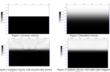
1. FD order and boundary condition
Figure 1 Accurate velocity Figure 2 Smoothed velocity
Figure 3 Updated velocity with second order normal grid and Clayton-Enquist boundary condition
Figure 4 Updated velocity with eight order staggered grid and PML boundary condition
Comparing figure 3 with figure 4, we find that the interface of velocity is already evident. The updated velocity in the figure 3 is not very stable, which appears many perturbations, and yet the result in figure 4 is better. There are no serious perturbations with velocity. It is proved that a better wavefield forward modeling is the basis of FWI.
2. The number of folds
The number of shot in figure 5 is ten and in figure 6 is fifty respectively and the interval of geophone is one grid point. It receives in all the surface. Comparing with them, we realize that the updated velocity is better within the large number of folds.
Figure 5 Updated velocity with ten sources Figure 6 Updated velocity with fifty sources
The number of shot in figure 7 and figure 8 is both twenty. The geophones are full covered with all the surface, but the interval in figure 7 is one grid point and in figure 8 is eight grid points. Both the convergent speed and effect of the former are superior to the latter. So we can know the same conclusion that the updated velocity is better within the large number of folds.
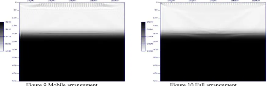
3. Array length and uniformity
The number of shot in figure 9 and figure 10 is both twenty distributed uniformly on the ground. But the difference is the received condition that the former’s geophone is mobile arrangement and the latter’s is full cover with the surface. Through comparison and analysis, it can be found that the accuracy and convergent speed of the latter are superior than the former’s. The reason is that the longer arrangement increases indirectly the folds. But we also can observe that the integrity and continuity of velocity interface is better, in addition the perturbations of updated velocity was smaller. This is because the mobile arrangement makes the energy of the folds more uniform, so the updated velocity is stable. According to the comprehensive analysis of above two situations, the more spread length can make updated velocity more accurate and make the result much better. At the same time uniform folds can bring out more stable result. So in the process of FWI, we should fully consider the effects of folds and arrangement length in observation system on the updated velocity, meanwhile it also should be pay attention the impact of uniformity on the stability.
Figure 9 Mobile arrangement Figure 10 Full arrangement
4. Dominant frequency of wavelet
The initial velocity model is the same as the above. The dominant frequency of wavelet in figure 11 is 10 Hz and figure 12 is 30 Hz. The latter’s effect is inferior to the former’s, which of the reason is that low frequency component represents the amount of long wavelength in the seismic wave. It can match the background velocity better to get the right gradient direction. So the convergence speed is faster and the
Figure 11 Updated velocity with 10 Hz Figure 12 Updated velocity with 30 Hz result is more stable and better. High frequency component represents the amount of short wavelength, in other words it presents tiny perturbation. It can be closer to the real value on the basis of accurate ground model. But for inaccurate ground model, the corresponding low frequency component is more favorable to updated velocity. So we should use low frequency wavelet in FWI firstly, then use high frequency again later. For frequency-division method, the FWI in frequency domain has been implemented effectively.
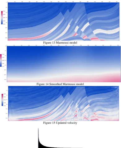
Marmousi model test
In order to test the modeling ability of FWI for the shallow and middle in complex geological conditions, the size of marmousi model we used in this article is 151 x767 points, As shown in figure 13. Figure 14 is the 10 times iteratively smoothing result of initial velocity model, where smooth parameters are 30 points interval for z direction and 40 points interval for x direction.
seen that with the increase of iterations, the smoothed model converges gradually in the right direction. The model is improved from the shallow to the deep little by little. Figure 16 shows that the misfit function is decreasing with iteration. Early change is bigger, so the main features of structural contour are described out. On the contrary the late is the improvement of the details for fine adjustment velocity.
II.
CONCLUSION
Based on the understanding of FWI, we can know that this method can play a good role in velocity modeling of shallow and middle. It can detect the low velocity interlayer which is unable to be discovered by conventional velocity analysis. Thus it provides a reliable tool for the near-surface velocity modeling.
According to the analysis of the main influential factors for FWI, we obtain that everyone of accurate wavefield propagation, low frequency of wavelet, and high folds, uniformity, log array of the field observation system can promotes much better updated velocity and quicker convergent speed. As a consequence, we can use this methods to seek low-velocity interlayer and construct accurate near-surface velocity model. With the deepening of this topic research, it’s reasonable for us to believe that velocity modeling of FWI will also apply for other imaging methods and actual production work.
Figure 13 Marmousi model
Figure 14 Smoothed Marmousi model
Figure 15 Updated velocity