Three-Dimensional Numerical Analysis of Shear Flow E
ff
ects on
MHD Stability in LHD Plasmas
∗
)
Katsuji ICHIGUCHI
1,2), Yashiro SUZUKI
1,2), Yasushi TODO
1,2), Masahiko SATO
1),
Timothée NICOLAS
1), Benjamin A. CARRERAS
3), Satoru SAKAKIBARA
1,2), Yuki TAKEMURA
1),
Satoshi OHDACHI
1,2)and Yoshiro NARUSHIMA
1)1)National Institute for Fusion Science, 322-6 Oroshi-cho, Toki 509-5292, Japan 2)SOKENDAI, The Graduate University for Advanced Studies, Toki 509-5292, Japan
3)Universidad Carlos III, 28911 Leganes, Madrid, Spain
(Received 27 November 2015/Accepted 25 February 2016)
Effects of poloidal shear flow on the stability of interchange modes in a Large Helical Device (LHD) con-figuration are numerically studied. Three-dimensional (3D) numerical codes are utilized for the equilibrium and stability calculations. A static equilibrium is employed and a model poloidal flow as a flux function is incorpo-rated in the initial perturbation. The results show that the initially applied flow can suppress the growth of the interchange mode if the flow is sufficiently large.
c
2016 The Japan Society of Plasma Science and Nuclear Fusion Research
Keywords: MHD stability, shear flow, 3D numerical simulation, heliotron, interchange mode DOI: 10.1585/pfr.11.2403035
1. Introduction
In the recent experiments in the Large Helical De-vice (LHD), a phenomenon similar to a locked mode was observed [1, 2]. In this case, the m = 1/n = 1 mode grows rapidly just after the mode rotation stops and causes a partial collapse of the profile in the electron tempera-ture. Here, mand n are the poloidal and toroidal mode numbers, respectively. This phenomenon indicates that the shear flow of the plasma may be a candidate which sup-presses the growth of the mode. Thus, we numerically study the effects of the shear flow on the magnetohydrody-namics (MHD) stability against the pressure driven modes in the LHD plasmas by utilizing three-dimensional (3D) numerical codes.
2. Numerical Procedure and Flow
Model
In order to investigate the effect of the plasma flow, we should analyze the stability of the equilibrium includ-ing the flow consistently. However, any 3D equilibrium calculation scheme consistent with a global flow has not yet been established. Hence, as the first step of this flow stability analysis, we employ a static equilibrium. Then, we set a model global flow in the initial perturbation of the dynamics calculation.
We use the HINT code [3] for the calculation of the static equilibrium. This code solves the equilibrium equa-tions in the cylindrical coordinates (R, φ,Z). Here,RandZ author’s e-mail: [email protected]
∗)This article is based on the presentation at the 25th International Toki Conference (ITC25).
are the horizontal and the vertical axes, respectively, andφ is the toroidal angle. We use the MIPS code [4] for the sta-bility calculation. This code solves the full MHD equations for the HINT equilibrium in the same cylindrical coordi-nates. We examine the linear stability and the nonlinear dynamics of perturbations in the equilibrium by following the time evolution of the plasma.
Here, we consider the global flow as a function of the flux surface. In this case, it is convenient to spec-ify the profile of flow components in a flux coordinate system (ρ, θ, φ). Here ρ is the label of magnetic flux, andθ is the poloidal angle that is simply determined as tanθ =Z/(R−Rcnt), whereRcntdenotes the major radius of the equilibrium magnetic axis. Then, the flow compo-nents can be given in the form ofV =(0,Vθ(ρ),Vφ(ρ)) in the coordinates.
Since the MIPS code solves the MHD equations in (R, φ,Z), we must obtain the components of V = (VR,Vφ,VZ) at each grid point. By utilizing the relations V· ∇Peq(ρ)=0 andVθ2=VR2+V
2
Z, we obtain VR =
1
A2
−1
R
∂Peq
∂φ ∂Peq
∂R Vφ±K
∂Peq
∂Z
(1) and
VZ =
1
A2
−1
R
∂Peq
∂φ ∂Peq
∂Z Vφ∓K
∂Peq
∂R
, (2)
where
A2=
∂ Peq ∂R 2 + ∂ Peq ∂Z 2 and K= ⎡ ⎢⎢⎢⎢⎢ ⎣A2V2
θ −
Vφ R
∂Peq
∂φ
2⎤
⎥⎥⎥⎥⎥ ⎦
1/2
.
(3)
c
2016 The Japan Society of Plasma
Here equilibrium pressurePeqis used for the label of the
flux instead ofρ. SinceVθandVφare given as the functions ofρ, we need to know the relation between the cylindrical and the flux coordinate systems. In order to obtain the re-lation, we utilize the fact that the input ofPeq is given as
the function ofρand the resultant value is obtained as the function of (R, φ,Z) in the HINT calculation. By taking the inverse of the function ofPeq(ρ) numerically, we
ob-tainρ=ρ(Peq(R, φ,Z)), which is used for the evaluation of
Vθ(ρ) andVφ(ρ) as the function of (R, φ,Z).
3. Equilibrium Calculation
We employ the LHD configuration withRax =3.6 m,
γc = 1.13. Here, Rax and γc are the horizontal
posi-tion of the vacuum magnetic axis and the parameter of the aspect ratio of the helical coils, respectively. In the equilibrium calculation, we assume the pressure profile of
Peq=P0(1−ρ2)(1−ρ8) and the axis beta ofβ
0=4%, where
ρdenotes the square root of the normalized toroidal mag-netic flux. Figure 1 shows the bird’s eye view of thisPeq. Figure 2 shows the summary of the equilibrium quantities. The
´
ι=1 surface is located in the plasma column, where´
ι is rotational transform. There exists a significant pressure gradient and Mercier stability is unfavorable (DI > 0) atthis surface.
We employ the profile ofVθsimilar to the experimen-tal result, which is given by
Vθ/VA=ln[10(1.1−ρ)] exp[−9(1−ρ)2](1−ρ8).
(4)
Fig. 1 Bird’s eye view of equilibrium pressure profile at the hor-izontally elongated cross section.
Fig. 2 Profiles of equilibrium pressure, rotational transform, Mercier index, and normalized poloidal flow.
The profile is also plotted in Fig. 2. A substantial shear flow is applied at the
´
ι = 1 surface. Hereafter, we iden-tify the value of the flow by the maximum value ofVθ/VA,where VA denotes the Alfvén velocity. We also assume
Vφ=0.
4. Stability Results
In the stability calculation, we add the poloidal shear flow to the input perturbation given by the random noise, and follow the time evolution of the plasma. In the present calculation, we assume the dissipation parameters so that the resistivity, the viscosity, and the perpendicular and the parallel heat conductivities areη/μ0 = 10−6, ν = 10−5,
κ⊥ =10−6, andκ =10−3, respectively. Each parameter is
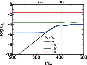
normalized byVARax. Figure 3 shows the time evolution of the total kinetic energy including the initial flow contri-bution. At first, we analyze the no flow caseVθ/VA=0 as a reference. In this case, an unstable mode grows linearly and is saturated att∼400τA, whereτAdenotes the Alfvén
time.
Next, we follow the time evolution of the plasma in the cases withVθ/VA=10−3, 10−2, and 10−1. In the case
of Vθ/VA = 10−3, the initial kinetic energy of the flow
Ek(flow) is much less thanEksat, whereEksatdenotes the
saturation level of the kinetic energy in the no flow case. The kinetic energy is constant up tot ∼ 300τA. This is
because the kinetic energy of the flow is much larger than that of the unstable mode in this region. The kinetic en-ergy increases beyondt ∼ 300τA, and shows almost the
same value as that of the no flow case beyondt ∼350τA.
In this region, the energy part of the unstable mode in the no flow case is superior to that of the initial flow. Thus, this initial flow is too small to affect the unstable mode.
In the case with Vθ/VA = 10−2, Ek(flow) is
compa-rable toEksat. The kinetic energy is almost constant and
slightly varies fort>400τAwhere the mode in the no flow
case is saturated. In the case withVθ/VA=10−1,E k(flow)
is much larger thanEksat. The kinetic energy is constant in the whole time region.
Figure 4 shows the mode pattern of the perturbed pressure ˜Prel at t = 320τA, which is defined as ˜Prel =
˜
P/max( ˜P), together with the puncture plot of the field lines. In the no flow case, the mode is in the linear phase at
Fig. 3 Time evolution of kinetic energy forVθ/VA =0, 10−3,
Fig. 4 Mode pattern of perturbed pressure ˜Prel and puncture
plots of field lines att = 320τA for (a)Vθ/VA =0, (b)
10−3, (c) 10−2, and (d) 10−1.
this time. The pattern shows the typical interchange mode. The mode numbers of the dominant component arem=4 andn=4, which are determined by the dissipation param-eters. In the case ofVθ/VA = 10−3, the mode pattern is
almost the same as that of the no flow case. In the case ofVθ/VA=10−2, the mode number of the dominant mode
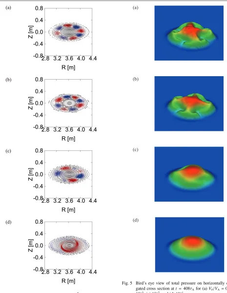
Fig. 5 Bird’s eye view of total pressure on horizontally
elon-gated cross section att =408τA for (a)Vθ/VA =0, (b)
10−3, (c) 10−2, and (d) 10−1.
reduces tom=2. This change of the mode number is sim-ilar to that due to the dissipation effects such as viscosity and heat conductivity. In the case ofVθ/VA = 10−1, any
explicit mode pattern cannot be recognized.
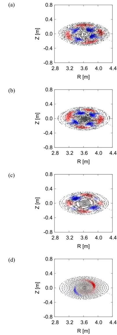
Figures 5 and 6 show the total pressure and the field line plots with ˜Prel att = 408τA in the saturation phase
Fig. 6 Mode pattern of ˜Preland puncture plots of field lines on a
horizontally elongated cross section att=408τAfor (a)
Vθ/VA=0, (b) 10−3, (c) 10−2, and (d)10−1.
significantly deformed so as to havem =4 structure and the field lines are stochastic in almost the entire plasma area. In the case ofVθ/VA =10−3, the behavior is almost
the same as that of the no flow case. The deformation of the pressure profile is slightly weaker and the field lines
are stochastic except for the peripheral region. In the case of Vθ/VA = 10−2, substantial stabilizing contribution to
the mode is seen. The deformation of the total pressure is much smaller than that of the no flow case. In addi-tion, the field lines are stochastic in the limited region. The nested surfaces remain in the wide region except around the surface. Also, the reduction in the mode number from
m=4 tom=2 indicates that the global shear flow stabi-lizes an interchange mode with higher mode numbers more effectively. In this nonlinear evolution, the mode rotation due to the flow is also observed explicitly. In the case of
Vθ/VA = 10−1, the stabilizing contribution is further
en-hanced. No change can be seen in the pressure profile and the flux surfaces also in the nonlinear region.
5. Summary
Effects of poloidal shear flow on the stability of inter-change modes in an LHD configuration are studied utiliz-ing 3D numerical codes. Static equilibrium is employed and a model poloidal flow is incorporated in the initial per-turbation. The effects of the shear flow are observed as follows:
No flow: The growth of an interchange mode leads to sig-nificant pressure collapse and field line stochasticity.
Ek(flow) Eksat: The flow does not interact with the
mode in the linear phase and slightly weakens the col-lapse and the stochasticity.
Ek(flow)∼Eksat: The flow reduces the mode number and
mitigates the collapse and stochasticity.
Ek(flow)Eksat: Explicit degradation is not seen in the
pressure profile and the magnetic surface structure. Thus, these results suggest that the initially applied model flow has an effect to suppress the growth of the interchange modes.
The initially applied flow in the present analysis causes the deviation from the force balance of the static equilibrium and induces a plasma motion due to the de-viation. Such motion can interact with the growth of the instability. Therefore, the present results does not exactly correspond to the stability property of the steady state with the flow. Nevertheless, the suppression of the mode makes us to expect the stabilizing contribution of the global flow also in the steady state. In order to confirm the stabiliz-ing contribution, we need to obtain the steady state firstly. For this purpose, we can utilize the result obtained with the present scheme, such as the final state of theVθ/VA=10−1
case. This analysis is planned as a future study together with the employment of the ExB rotation in modeling the flow.
Acknowledgments
26-04728 and 15k06651. The super computers Plasma Simulator in NIFS and Helios in the Computational Simulation Center of the International Fusion Energy Research Center (IFERC-CSC) were utilized for the numerical calculations.
[1] Y. Takemuraet al., Nucl. Fusion52, 102001 (2012).
[2] S. Sakakibara et al., Plasma Phys. Control. Fusion 55,
014014 (2013).
[3] Y. Suzukiet al., Nucl. Fusion46, L19 (2006).