Synthetic learning machines

(1)

M E T H O D O L O G Y

Open Access

Synthetic learning machines

Hemant Ishwaran

1*?

and James D Malley

2?

*Correspondence:

[email protected] ?_{Equal contributors}

1Division of Biostatistics, University of Miami, 1120 NW 14th Street, Miami, FL 33136, USA Full list of author information is available at the end of the article

Abstract

Background: Using a collection of different terminal nodesize constructed random forests, each generating a synthetic feature, a synthetic random forest is defined as a kind of hyperforest, calculated using the new input synthetic features, along with the original features.

Results: Using a large collection of regression and multiclass datasets we show that synthetic random forests outperforms both conventional random forests and the optimized forest from the regresssion portfolio.

Conclusions: Synthetic forests removes the need for tuning random forests with no additional effort on the part of the researcher. Importantly, the synthetic forest does this with evidently no loss in prediction compared to a well-optimized single random forest.

Keywords: Machine, Nodesize, Random forest, Trees, Synthetic feature

Background

Earlier work has shown how to optimally combine a set of predictors?classifier or probability machines?into a so-called regression collective[1]. Consider, for example, a collection of statistical learning machines chosen by the researcher, from subject matter knowledge or with statistical aspirations. It could contain versions of SVMs [2] with dif-ferent kernels, variants of the lasso [3], a group of neural nets [4], a collection ofk-nearest neighbors [5] with varyingk, along with several random forests [6]. The thought here is that each or several of these machines might be optimal for the data at hand, but tuning each and adjudicating the multiple outcomes and performances introduces a second layer of statistical and data analytic overhead. Instead, a prefered way to proceed is to use a regression collective which optimally combines machines, thus avoiding the difficulty of individual machine tuning.

This new method [1], whose R code is abbreviated COBRA (for COmBined Regres-sion Alternative), is just this kind of combining method. It has the property, that in the limit of large data, it is at least as good as the best predictor in the collection, and gen-erates its prediction without having to declare which of the individual predictors might be optimal for the data at hand. For example, on a given data set one method might be Bayes optimal for classification given enough data, and on another data set another machine might be optimal. In all cases the regression collective, given enough data, is Bayes optimal if any one machine is so, and where this unnamed optimal machine in the portfolio of the collective can vary over data sets. The method achieves this optimality

(2)

for any data, with a possibly large number of features with mixed category or contin-uous features and arbitrary correlation structure. As a practical matter the regression collective requires no tuning of the individual machines on the part of the researcher: the method is entirely nonparametric and model-free. As one detail, there is no require-ment for specific and correct interaction terms, however defined, as input for the method. Instead, machines that include such interaction terms can be added to the portfolio of the collective.

The COBRA method is not a committee or ensemble method, nor is it a voting method. It is closer to ak-nearest neighbor scheme. However the distance function, or metric, for measuring closeness in the collective is not Euclidean distance or any weighting thereof, but a method that uses the multiple predictions of the several component machines to access closeness of a test data point to the training data. For each training data point, one checks if its predicted value under a given machine is close to the predicted value of the test data point under that same machine, and if closeness holds for a majority of the machines, then that training point is deemed close to the target test data point, otherwise it is deemed distant. The final prediction for the test data point is a sum of the training data outcomes using only those data points that are close. In particular this means pre-dictions from the several machines are not averaged to make the prediction on the test case, but rather the predicted value is a weighted average of the original outcomes. That is, COBRA is a type of locally weighted averaged estimator.

While the example above of a regression collective over a set of learning machines was the motivation for COBRA [1], it has also lead to increased scrutiny of analytic approaches using collections of features, biologically grounded networks or pathways each as new inputs to other machines. Here the separate networks are used as inputs to the various machines within the collective [7]. Then, using the machines built from these networks assynthetic features, they can be sent to a suitable learning machine for which it is then possible to compare and evaluate the predictive capacity and interactions between the networks: Are some networks better than others in the portfolio? In what subset of the data might that be true?

(3)

Methods

Random Forests [6] (hereafter abbreviated as RF), is an ensemble learning method which calculates ensemble predicted value by aggregating a collection ofntree ≥ 1 randomly grown trees. In multiclass problems, averaging the terminal node relative frequency of class labels over a forest of random classification trees yields ensemble predicted prob-abilities for each class label, while in regression problems, averaging the terminal node mean value yields ensemble predicted values for theY-response. Equivalently, one can show that the resulting ensemble predicted value of a RF can be written as weighted convex combination of outcomes. Thus, RF is a locally weighted averaging estimator. A unique feature of RF trees are that they are random in the following sense: a) Each tree is grown using an independent bootstrap sample (i.e. a sample drawn with replacement from the original data set, of sizenequal to the original sample size); (b) Random fea-ture selection is employed in which at each node of the tree during the tree growing process, a random subset of 1 ≤ mtry ≤ pfeatures are selected, wherepequals the total number of features, and the node is split using the variable from themtry candi-date variables having the best split. Splitting of a RF tree is repeated recursively, with the tree grown as far as possible until it is no longer possible to identify groups that differ on the outcome, or the sample size at that node is too small. Terminal node sizes (the ends of the tree) satisfy the condition that they contain a minimum ofnodesize ≥ 1 unique cases.

Of the three tuning parameters used by RF,(ntree, mtry, nodesize), optimal tuning of nodesize has the greatest potential to improve prediction performance. This is because nodesize acts as a type of bandwidth parameter that controls the level of smoothing of the RF predictor. It has now become apparent to the machine learning community that the optimal choice fornodesize depends heavily on the underyling data. In large nsample settings for example, it is generally believed thatnodesize should be large to ensure good performance. Rationale for this comes from large sample asymptotics which requirenodesize to increase to∞in order to ensure consistency. Results of this nature have for example been used to establish Bayes-risk consistency for RF classification [8]. On the other hand, in high-dimensional problems involving a large number of features, the opposite has been observed, with performance generally improving with decreasing nodesize [9]. In studying lower bounds for the rate of convergence in RF regression, it has been shown that rates of convergence improve whennodesize is small when the number of featurespexceeds the sample sizen[10].

(4)

Algorithm 1 Synthetic Random Forests (SRF)

1: Choose a set of candidate nodesize valuesN = {n1,n2,. . .,nD}.

2: Fit a RF withnodesize= njforj =1,. . .,D. Use the samentree and mtry value for

each forest. Denote the resulting forests by RF1,. . ., RFD.

3: Calculate the predicted value for each random forest RFj,j = 1,. . .,D. We call the predicted value the synthetic feature.

4: Fit a RF using for features both the newly created synthetic features and the originalp

features (using the samentree and mtry value as before). We call this the synthetic RF.

Remarks

Implementing SRF conveniently involves doing nothing more than fitting a RF to a slightly expanded set of features, which includes in addition to the originalpfeatures, a new col-lection of synthetic features obtained by fitting RF under differentnodesize values. While conceptually straightforward, there are some important points to keep in mind when implementing SRF:

1. The dimension of a synthetic feature can be one or greater. In regression, the synthetic feature is the predicted value of theY-response, which is

one-dimensional, however in multiclass problems, the synthetic feature is the predicted probability of the class label. If there areJclasses, this yields a

J-dimensional synthetic feature. Note that since the predicted probabilities are linearly dependent as they sum to 1, we discard by convention the last coordinate and use only the firstJ? 1predicted probabilities.

2. To avoid overfitting, when constructing the synthetic feature, we use out-of-bag (OOB) predicted values. In a bootstrap sample only 63.2% of the data is used on average (due to sampling with replacement), leaving 36.7% of the data untouched. This latter data is termed OOB because it is out of sample and can be used to calculate OOB ensemble predicted values. The OOB predicted value for each data pointXdoes not use theY-response forXand therefore represents a

cross-validated out-of-sample estimate.

3. The values ofntree and mtry are kept fixed throughout. Selecting a reasonable value forntree is not difficult and performance is robust to its choice?as long as its value is kept reasonably large, say 250 or more. Optimizing overmtry can improve RF but we have found that creating synthetic features by varying bothmtry and nodesize values can sometimes negatively impact performance of SRF. We find keepingmtry fixed at default values and constructing synthetic features by varying nodesize works very well.

4. Another reason for favoring optimization ofnodesize rather than mtry is its granularity. Fornodesize, regardless ofnorp, it suffices to consider a handful of small values, a few intermediate values, and a few large values in the optimization (in the case of largen, the rate at whichnodesize converges to∞, required for consistency, can be far slower thann; thus relatively small values ofnodesize can be used even whennis relatively large). In contrast, optimization overmtry depends uponp, which creates not only an expensive optimization problem in

(5)

Results

We compared the performance of four methods, RF, RFopt, SRF, and COBRA over a col-lection of regression and multiclass benchmark datasets. The four methods were defined as follows:

1. SRF denotes Synthetic Random Forests described in Algorithm 1. Values for nodesize were set atN = {1, 2, 3, 4, 5, 6, 7, 8, 9, 10, 20, 30, 50, 100}. The synthetic RF of line 4 was calculated usingnodesize=5. While this value can be included as a user parameter for SRF, we found that changing its value did not alter our findings very much. Thus we chose not to cloud our findings and instead opted for a fixed value ofnodesize=5throughout our simulations.

2. RF denotes a standard forest calculated usingnodesize=5. The samenodesize value was used as for the synthetic forest in SRF in order to assess the efficacy of the synthetic features. If the synthetic features are not used in node splitting of a synthetic forest, the resulting forest should closely approximate a regular forest, and thus performance of SRF should closely approximate performance of RF. 3. RFopt denotes the forest calculated using the optimal nodesize fromN .

Specifically: the optimal nodesize was defined as the nodesize valuenjfrom theRFj forest with the smallest OOB error in SRF. We include RFopt to assess whether a globally nodesize-optimized forest can compete with the locally

nodesize-optimized synthetic forest.

4. COBRA implements the aggregation method described in [1]. For regression machines required as input to COBRA we used the same{RFj}D₁ machines used by SRF. Using the same synthetic features as SRF allows us to assess the effectiveness of arbitrary convex combination weighting used by RF compared with zero-one weighting used by COBRA. As a side note, we also tried implementing COBRA using the default machines that comes with its code (lasso, ridge regression, SVM and random forests) to assess whether a generic COBRA implementation compared favorably to SRF. However, the results were so unfavorable that we excluded them from our findings.

(6)

Regression results

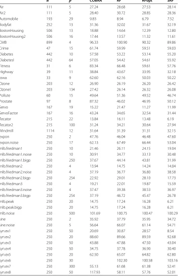
A large collection of regression datasets was used to assess the performance of each method (Table 1). Datasets with a capital identify real data while those in lower case

Table 1 Regression benchmark performance

n p COBRA RF RFopt SRF

Air 111 5 27.24 28.68 27.53 28.14

Air2 111 5 28.40 30.72 28.85 28.36

Automobile 193 29 9.83 8.94 6.79 7.52

Bodyfat 252 13 31.36 32.02 31.67 32.19

BostonHousing 506 13 18.88 14.64 12.39 12.80

BostonHousing2 506 16 17.44 13.57 11.32 11.61

CMB 899 4 96.33 100.90 90.32 89.86

Crime 47 15 61.74 59.99 59.51 59.03

Diabetes 442 10 57.58 53.22 53.14 55.20

DiabetesI 442 64 57.05 54.42 54.61 55.92

Fitness 31 6 83.34 66.48 59.61 57.76

Highway 39 11 38.84 43.67 33.95 32.18

Iowa 33 9 62.60 62.16 50.03 50.22

Ozone 203 12 26.90 26.19 26.20 26.42

OzoneI 203 134 27.42 26.14 26.32 26.08

Pollute 60 15 49.64 51.36 49.52 46.74

Prostate 97 8 87.32 46.02 46.95 50.12

Servo 167 19 15.22 21.47 11.27 11.99

ServoFactor 167 16 43.24 34.65 32.54 31.44

Tecator 215 22 13.84 16.11 13.48 6.19

Tecator2 215 100 31.24 34.21 30.64 27.94

Windmill 1114 12 31.64 31.39 31.31 32.15

expon 250 2 47.76 46.04 46.48 47.60

expon.noise 250 17 62.13 67.49 66.44 53.04

mlb.friedman1 250 10 21.46 26.11 24.15 19.04

mlb.friedman1.noise 250 10 30.91 34.77 33.13 30.48

mlb.friedman1.bigp 250 250 37.67 44.14 43.81 31.99

mlb.friedman2 250 4 13.94 14.75 14.24 14.04

mlb.friedman3 250 4 19.21 22.01 19.87 15.59

mlb.peak 250 20 14.75 17.24 16.28 6.21

mlb.peak.bigp 250 20 14.75 17.24 16.28 6.21

mlb.noise 250 500 101.69 100.75 100.47 100.29

sine 250 2 35.92 37.79 35.95 34.72

sine.noise 250 5 56.64 66.07 61.14 54.71

syn.ex1 250 50 20.69 30.87 28.57 8.54

syn.ex2 250 20 88.60 89.66 89.59 92.68

syn.ex3 250 50 43.88 47.88 47.50 43.04

syn.ex4 250 50 34.75 37.78 36.90 30.40

syn.ex5 250 20 62.50 65.07 64.82 62.80

syn.ex6 250 30 102.30 100.58 103.16

syn.ex7 250 300 55.13 61.68 61.38 52.41

syn.ex8 250 50 117.93 58.11 57.76 52.01

(7)

are synthetic data. Many of the synthetic data were obtained from the mlbench R-package [14] and are labeled starting with ?mlb?. In total, 46 datasets were used with sample sizes varying fromn=31 ton=1114; number of features varied fromp=2 to p=500. Sample sizes for synthetic data were set atn=250.

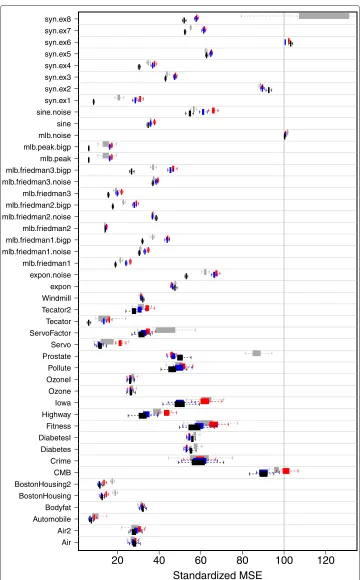
Performance was assessed using standardized mean-squared error (MSE) defined as MSE divided by the variance of theY-response and multiplied by 100. Standarized MSE facilitates comparison across datasets: a value of 100 can be used as a benchmark value. For real data, MSE was calculated using 10-fold cross-validation. For synthetic data, MSE was evaluated by using an independent test-set of sizen=5000. The entire process was repeated independently 100 times. Table 1 reports the averaged standardized MSE from the 100 replicates. Figure 1 displays the 95% confidence regions of standardized MSE.

Table 1 and Figure 1 show clear superiority of SRF, especially over synthetic data. To formally assess performance differences we used univariate and multivariate nonpara-metric statistical tests [15]. To compare two methods we used the Wilcoxon signed rank test applied to the difference of their standardized MSE values. The exact p-value for the Wilcoxon signed rank test are recorded along the upper diagonals of Table 2. The lower diagonal values record the corresponding test statistic where small values indicate a difference. To test for an overall difference among procedures we used the Iman and Dav-enport modified Friedman test [15]. For each dataset, the performance of each method was ranked from 1 through 4, and the average of these ranks over all datasets for each procedure calculated. The diagonal values of the table record this average rank which was used for the Friedman test. This latter test yielded a near-zero p-value, thus provid-ing strong evidence of difference between methods. Overall, SRF is ranked first, followed by RFopt, COBRA, and then RF. Wilcoxon p-values provide strong evidence supporting superiority of SRF to each of the three other methods.

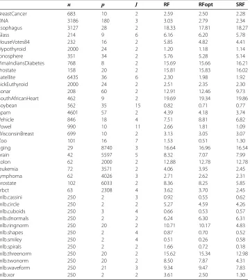
Multiclass results

To further assess the performance of SRF, a total of 38 multiclass benchmark datasets were used. Sample sizes ranged fromn = 29 ton = 6435; features varied fromp = 2 top= 8740; and number of classesJvaried fromJ = 2 toJ = 15 (Table 3). The same nomenclature was adopted as in our regression experiment. Real datasets are indicated with capitals and synthetic data frommlbenchare labeled starting with ?mlb?. Datasets ?aging?, ?brain?, ?colon?, ?leukemia?, ?lymphoma? and ?srbct? are well-known benchmark microarray datasets (note howpnin each of these).

(8)

20

40

60

80

100

120 Standardized MSE

Air Air2 Automobile Bodyfat BostonHousing BostonHousing2 CMB Crime Diabetes DiabetesI Fitness Highway Iowa Ozone OzoneI Pollute Prostate Servo ServoFactor Tecator Tecator2 Windmill expon expon.noise mlb.friedman1 mlb.friedman1.noise mlb.friedman1.bigp mlb.friedman2 mlb.friedman2.noise mlb.friedman2.bigp mlb.friedman3 mlb.friedman3.noise mlb.friedman3.bigp mlb.peak mlb.peak.bigp mlb.noise sine sine.noise syn.ex1 syn.ex2 syn.ex3 syn.ex4 syn.ex5 syn.ex6 syn.ex7 syn.ex8

Figure 1 Regression benchmark results.Cross-validated and test-set standardized mean-squared error (MSE) performance over 100 independent replications. Boxplots display results from the 100 replications for COBRA (gray square symbol), RF (red square symbol), optimized random forestsRFopt(blue square symbol), and synthetic random forests SRF (). Standardized MSE obtained by dividing MSE by the variance of the

(9)

Table 2 Regression benchmark performance

COBRA RF RFopt SRF

COBRA 2.7 0.0968 0.3703 0.0000

RF 388 3.3 0.0000 0.0000

RFopt 623 1029 2.3 0.0018

SRF 1005 966 827 1.7

Upper diagonal values are Wilcoxon signed rank p-values comparing two procedures; lower diagonal values are the corresponding test statistic. Diagonal values (in bold) record the overall rank of a procedure.

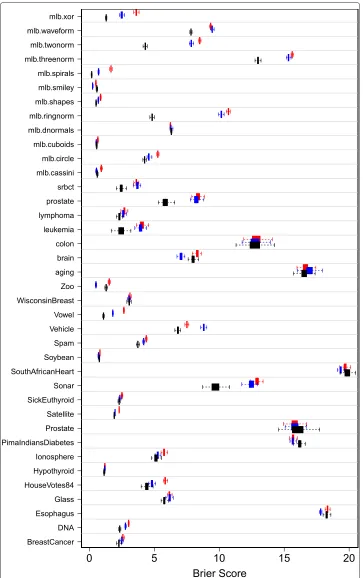
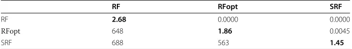
Table 3 and Figure 2 show superiority of SRF to the three other methods. As in the regression experiment, performance differences are especially noticeable over syn-thetic data. Noticeable performance differences are also observed over certain microarray datasets (srbct, prostate, and leukemia). Table 4 displays results of nonparametric tests comparing procedures. The results parallel those of Table 2: SRF has best overall rank and there is strong evidence of its superiority. The modified Friedman test of equality

Table 3 Multiclass benchmark performance

n p J RF RFopt SRF

BreastCancer 683 10 2 2.59 2.50 2.28

DNA 3186 180 3 3.03 2.79 2.34

Esophagus 3127 28 2 18.33 17.81 18.27

Glass 214 9 6 6.16 6.20 5.78

HouseVotes84 232 16 2 5.85 4.82 4.41

Hypothyroid 2000 24 2 1.20 1.18 1.14

Ionosphere 351 34 2 5.76 5.28 5.14

PimaIndiansDiabetes 768 8 2 15.69 15.66 16.21

Prostate 158 20 2 15.81 15.83 16.02

Satellite 6435 36 6 2.30 1.98 1.92

SickEuthyroid 2000 24 2 2.51 2.35 2.30

Sonar 208 60 2 12.91 12.46 9.73

SouthAfricanHeart 462 9 2 19.69 19.34 19.86

Soybean 562 35 15 0.82 0.71 0.77

Spam 4601 57 2 4.39 4.18 3.74

Vehicle 846 18 4 7.51 8.81 6.82

Vowel 990 10 11 2.66 1.81 1.09

WisconsinBreast 699 10 2 3.13 3.05 3.07

Zoo 101 16 7 1.53 0.51 1.30

aging 29 8740 3 16.64 16.96 16.54

brain 42 5597 5 8.32 7.07 7.99

colon 62 2000 2 12.88 12.78 12.78

leukemia 72 3571 2 4.06 3.95 2.45

lymphoma 62 4026 3 2.71 2.62 2.31

prostate 102 6033 2 8.36 8.25 5.85

srbct 63 2308 4 3.62 3.70 2.45

mlb.cassini 250 2 3 0.92 0.55 0.62

mlb.circle 250 2 2 5.27 4.59 4.26

mlb.cuboids 250 3 4 0.66 0.53 0.57

mlb.dnormals 250 2 2 6.24 6.30 6.31

mlb.ringnorm 250 20 2 10.71 10.17 4.83

mlb.shapes 250 2 4 0.87 0.70 0.52

mlb.smiley 250 2 4 0.51 0.26 0.58

mlb.spirals 250 2 2 1.66 0.72 0.18

mlb.threenorm 250 20 2 15.62 15.34 12.98

mlb.twonorm 250 20 2 8.50 7.87 4.31

mlb.waveform 250 21 3 9.34 9.47 7.83

mlb.xor 250 2 2 3.61 2.50 1.30

(10)

0

5

10

15

20 Brier Score

BreastCancer DNA Esophagus Glass HouseVotes84 Hypothyroid Ionosphere PimaIndiansDiabetes Prostate Satellite SickEuthyroid Sonar SouthAfricanHeart Soybean Spam Vehicle Vowel WisconsinBreast Zoo aging brain colon leukemia lymphoma prostate srbct mlb.cassini mlb.circle mlb.cuboids mlb.dnormals mlb.ringnorm mlb.shapes mlb.smiley mlb.spirals mlb.threenorm mlb.twonorm mlb.waveform mlb.xor

(11)

Table 4 Multiclass benchmark performance

RF RFopt SRF

RF 2.68 0.0000 0.0000

RFopt 648 1.86 0.0045

SRF 688 563 1.45

Upper diagonal values are Wilcoxon signed rank p-values comparing two procedures; lower diagonal values are the corresponding test statistic. Diagonal values (in bold) record the overall rank of a procedure.

of procedures yielded a near zero p-value, further confirming evidence of SRF?s superior performance.

Conclusions

Peering more closely at synthetic forests it is possible to discern a reason for the generally good performance of any RF. That is, a single RF is acting as a synthetic machine across all the features, where each original feature is effectively a stand-alone synthetic feature. The manner in which RF synthesizes its features also plays a vital role in its success. RF forms its predictor by taking a locally weighted convex combination of the outcomes. Importantly, this differs from the COBRA method, which locally weights the outcomes using zero-one weights. The superior performance of synthetic forests to COBRA found in our experiments, even when using the same synthetic features as individual, separate constituents in the collective portfolio, suggests that the use of convex, locally determined weights may play a key role in its success, and where these weights are chosen by the refined cells in the data space that are given by the terminal nodes in each tree in each forest.

Performance gains for synthetic forests were most noticeable among the simulated data in our benchmark experiments. We believe the reason for this is that these particular data structures have high signal and sparse solutions. The synthetic random forest, by vary-ing the synthetic inputs over a wide range of user-specified terminal node sizes, acts as a local smoothing optimizer. Our results suggest such tuning is better able to handle high signal, sparse data. Indeed, especially noteworthy given this outcome, is that such data are known to be especially challenging and are likely to constitute a significant fraction of increasingly available big data sets. Another important practical implication of synthetic forests is that the number of RF user tuning parameters are greatly minimized. Most importantly, the synthetic forest does this with evidently no loss in prediction compared to a well-optimized single random forest.

Finally, and more comprehensively, the results here suggest that any statistical learning machine, Super X say, that has user tuning parameters, or indeed required parameter estimation, can be deployed as a Synthetic Super X using RF, with less overhead and likely no real loss in predictive capacity over the fully optimized Super X on the given data.

Abbreviations

COBRA: COmBined regression alternative; RF: Random forests;RFopt: Nodesize optimized random forests; SRF: Synthetic random forests.

Competing interests

The authors declare that they have no competing interests.

Authors? contributions

(12)

Acknowledgements

HI was funded by DMS grant 1148991 from the National Science Foundation and grant R01CA163739 from the National Cancer Institute. JDM was supported by the Intramural Research Program at the National Institutes of Health. The authors thank the referee of the paper for their wonderfully helpful comments.

Author details

1_{Division of Biostatistics, University of Miami, 1120 NW 14th Street, Miami, FL 33136, USA.}2_{Center for Information}

Technology, National Institutes of Health, Bethesda, MD 20892, USA.

Received: 25 June 2014 Accepted: 18 November 2014

References

1. Biau G, Fischer A, Guedj B, Malley JD:COBRA: a non-linear aggregation strategy.Paris ? France: Technical Report, Universit? Pierre et Marie Curie; 2013:1?27. [http://www.lsta.upmc.fr/BIAU/publications.html]

2. Vapnik V:Statistical Learning Theory. New York: Wiley; 1998.

3. Tibshirani RJ:Regression shrinkage and selection via the lasso.J R Stat Soc Series B1996,58:267?288. 4. Ripley DB:Pattern recognition and neural networks. Cambridge: Cambridge University Press; 1996. 5. Cover TM, Hart PE:Nearest neighbor pattern classification.IEEE Trans Inform Theory1967,IT-13:21?27. 6. Breiman L:Random forests.Mach Learn2001,45:5.

7. Pan Q, Hu T, Malley J, Andrew A, Karagas M, Moore J:A system-level pathway-phenotype association analysis using synthetic feature random forest.Genet Epidemiol2014,38(3):209?219.

8. Biau G, Devroye L, Lugosi G:Consistency of random forests and other averaging classifiers.J Mach Learn Res 2008,9:2015?2033. [http://doi.acm.org/10.1145/1390681.1442799]

9. Ishwaran H, Kogalur UB, Chen X, Minn AJ:Random survival forests for high-dimensional data.Stat Anal Data Mining2011,4:115?132. [http://dx.doi.org/10.1002/sam.10103]

10. Lin Y, Jeon Y:Random forests and adaptive nearest neighbors.J Am Stat Assoc2006,101(474):578?590. 11. Ishwaran H, Kogalur U:Random forests for survival, regression and classification (RF-SRC), R package version

1.5.5.2014. [http://cran.r-project.org/web/packages/randomForestSRC/index.html] 12. Liaw A, Wiener M:Classification and regression by randomforest.R News2002,2(3):18?22.

13. Guedj B:COBRA: nonlinear aggregation of predictors. R package version 0.99.4.2013. [http://cran.r-project. org/web/packages/COBRA/index.html]

14. Leisch F, Dimitriadou E:mlbench: machine learning benchmark problems. R package version 2.1-1.2012. [http://cran.r-project.org/web/packages/mlbench/index.html]

15. Demsar J:Statistical comparisons of classifiers over multiple data sets.J Mach Learn Res2006,7:1?30. [http://www.jmlr.org/papers/v7/demsar06a.html]

doi:10.1186/s13040-014-0028-y

Cite this article as:Ishwaran and Malley:Synthetic learning machines.BioData Mining20147:28.

Submit your next manuscript to BioMed Central and take full advantage of:

? Convenient online submission

? Thorough peer review

? No space constraints or color ?gure charges

? Immediate publication on acceptance

? Inclusion in PubMed, CAS, Scopus and Google Scholar

? Research which is freely available for redistribution