R E S E A R C H
Open Access
Microarray enriched gene rank
Eugene Demidenko
Correspondence: [email protected] Department of Biomedical Data Science, Institute for Quantitative Biomedical Sciences, Geisel School of Medicine at Dartmouth, Hanover, NH 03755, USA
Abstract
Background: We develop a new concept that reflects how genes are connected based on microarray data using the coefficient of determination (the squared Pearson correlation coefficient). Our gene rank combines a priori knowledge about gene connectivity, say, from the Gene Ontology (GO) database, and the microarray
expression data at hand, called the microarray enriched gene rank, or simply gene rank (GR). GR, similarly to Google PageRank, is defined in a recursive fashion and is
computed as the left maximum eigenvector of a stochastic matrix derived from microarray expression data. An efficient algorithm is devised that allows computation of GR for 50 thousand genes with 500 samples within minutes on a personal computer using the public domain statistical package R.
Results: Computation of GR is illustrated with several microarray data sets. In particular, we apply GR (1) to answer whether bad genes are more connected than good genes in relation with cancer patient survival, (2) to associate gene connectivity with cluster/subtypes in ovarian cancer tumors, and to determine whether gene connectivity changes (3) from organ to organ within the same organism and (4) between organisms.
Conclusions: We have shown by examples that findings based on GR confirm biological expectations. GR may be used for hypothesis generation on gene pathways. It may be used for a homogeneous sample or for comparison of gene connectivity among cases and controls, or in longitudinal setting.
Introduction
The key element of Google’s success is the PageRank that determines the order of web-pages displayed for a keyword search. The original algorithm by Pageet al.[1] received considerable attention. The idea to use the PageRank to rank genes with respect to their connection to other genes seems obvious and indeed is not new: GeneRank developed by Morrison et al.[2] is a straightforward generalization of PageRank of Google. Two versions of GeneRank are suggested: (1) using GO annotation or (2) Pearson correlation coefficient, r. In both cases, the entries of the connectivity matrix are binary: 0 genes are not connected and 1 if genes are connected. In the correlation version (2), the genes defined connected if r > 0.5. Both versions suffer from series limitations: (1) The GO annotation version is difficult to realize in practice because, e.g. withn=50, 000 number of genes one has to fill in the connectivity matrix with 2.5×10⁹elements. Moreover, since the set of genes varies from study to study and from organ to organ, the researcher faces a daunting problem with every new set of microarray experiments. (2) The correlation
version brushes off negative correlations which may be very important, and the thresh-old 0.5 has no justification. The gene rank we suggest is free of these shortcomings: (1) it combines GO library with correlation so that only the connectivity of a small proportion of genes can specified, (2) no thresholding is applied since we use the squared correlation coefficient (coefficient of determination).
The goal of this work is to equip the researcher with a new concept, microar-ray enriched gene rank (GR), that combines a priori knowledge about gene con-nectivity with researcher-derived microarray data, and can be computed on his/her own personal computer with as many as 50,000 genes and 500 samples within few minutes.
Traditional gene ranking methods using microarray data are based on ordering of t-statistics (or respective p-values) when the means between cases and controls are compared, or in a more general case, when the microarray sample is correlated with a phe-notype, see Winteret al. [3], Zuberet al.[4]. Much of the literature studies issues related to minimization of the false discovery rate or correlation between genes; see Opgen-Rhein et al.[5], Nitschet al.[6], Masoudi-Nejadet al.[7]. We, however, consider the gene con-nectivity problemregardlessof the phenotype. The assumption of the present work is that gene connectivity can be adequately expressed in terms of the gene pairwise squared cor-relation matrix, therefore the phenotype is not required. However, the association with phenotype or disease status can be examined further, such as through comparison of GRs between controls and cases.
GR reflects the complexity of genetic organization and is illustrated with several existing microarray data sets. This new genetic quantity gives rise to new biological insights, such as connectivity within clusters/subtypes, between organs within the same organism, and between organisms. GR can be used to discover gene pathways and track those under different experimental conditions or time wise.
Methods
We assume that the gene expression data are presented as ann×mmatrix, where rows are genes (the number of rows equaln)and columns are samples (the number of sam-ples/conditions equalsm). Hereafter, we use boldface to denote vectors and matrices, and the subscript ito indicate the ith gene andj to indicate thejth sample. It is assumed that, for each genei, the sample{xij,j= 1, 2,. . .,m}consists of independent identically distributed (iid) observations (microarray measurements); moreover,nsamples belong to a multivariate normal distribution. In practice, we may apply a nonlinear transforma-tion, such as the log-transformatransforma-tion, to avoid skewness, when it is appropriate—say, when observations are positive. Under these assumptions, then×npairwise Pearson correla-tion matrix computed from the matrix data,R= {rij}, is an appropriate measure of genes connectivity; the negative values indicate negative relationships and the positive values indicate positive connectivity. Our concern is the gene connectivity regardless of the neg-ative or positive relationship, so the squared correlation coefficient, or the coefficient of determination, should be used. In fact, the squared correlation coefficient is more inter-pretable in the statistical sense than the traditional correlation coefficient. Namely, rij2 indicates the proportion of the variance of theith gene explained by thejth gene and vice verse
rij2=rji2
The premise of this work is that the gene network is represented by ann×nmatrix of squared correlation coefficients,R2 =
r2ij
. In the terminology of Langfelder and Horvath [8], matrixR2is called the co-expression network withβ = 2. Note thatR2is treated as the whole mathematical object, not the matrix product ofRand itself. The sum ofrij2in theith row of matrixR2is an indication of gene connectivity. However, in order to compare genes from different rows, we need to normalize them so that the sum in each row is one. That leads us to the normalized squared correlation coefficient,
r∗2ij= r 2
ij n
k=1rik2
. (1)
The n×nmatrix with these entries will be referred to as the normalized squared correlation matrixR2∗. MatrixR2∗belongs to the family ofstochastic matrices: All elements are nonnegative and the sum of elements in each row is one.
Now letpjrepresent the rank of genej. Another way to compute the gene connectivity is to use the weighted sum of squared correlations with weightspi:ni=1pir2∗ij. This means that the squared correlations are weighted with respect to the connectivity and as in the PageRank, leads to a recursive definition ofp. Let the nonnegative and less or equal to oneajbe thea priorigenejconnectivity measure, 0≤aj ≤1. Ifaj =0, gene expression data adds nothing toa prioriconnectivity; ifaj=1, then the connectivity is solely derived from the expression data. Measureajmay represent our biological knowledge about gene connectivity, or it may be a noninformativea prioridistribution frequently used in the Bayesian approach, Gelmanet al.[9].
Finally, the recursive definition of the microarray enriched gene rank is:
pj= 1
n(1−aj)+aj n
i=1
pir∗2ij, j=1, 2,. . .,n. (2)
The first term on the right-hand side,(1−aj)/n, represents oura prioriknowledge about the connectivity of genej. The second term,ajpir∗2ij, represents the connectiv-ity derived from the gene expression data at hand. Sincepjcombinesa prioriknowledge about gene connectivity with microarray data experiments, we call it the microarray enriched gene rank, or simply gene rank (GR).
In matrix language, Equation (2) can be expressed asp=Hp, wherepis then×1 vector of gene ranks,is the matrix transposition symbol, andHis then×nmatrix
H=1
n(1−a)1
+AR2
∗, (3)
where1is then×1 vector of ones,ais then×1 vector of{aj,j = 1, ..,n}, andAis the n×ndiagonal matrix withaon the diagonal,A=diag(a).
Definition 1.The gene rank (GR) vector is the maximum left eigenvector of matrixH: the n×1vectorpthat satisfies the equation
p=Hp.
positive elements in our case, this eigenvalue is maximum and other eigenvalues are pos-itive but smaller than one. Hereafter, we refer to GR as the left maximum eigenvector of matrixH. In a special case when all gene connectivities area prioriset to zero, we have aj=1 and the GR of genejis proportional to the sum of squared correlations in rowj. In our computations below, we assume the noninformative prior connectivity distribution, aj=0.9=const (Google usesaj=0.85). Our results reported below are fairly robust to the choice of this constant due to largen.
Whennis of the order of a few thousands, standard methods of eigenvector compu-tation may be used. Several authors suggest efficient algorithms for compucompu-tation of the maximum left eigenvector of a stochastic matrix (Golub and Greif [11], Wuet al.[12]). However, whennis of the order of tens of thousands, new algorithms are required because even storing the squared correlation matrix is problematic. An efficient method for com-putation of GR using a public domain statistical packageRdoes not require storingR2
and is outlined in the online methods with theR[13] script provided. For example, com-putation of GR for a microarray data with 50,000 genes and 500 samples takes only few minutes on a personal computer.
Gene rank and cluster analysis
Cluster analysis is a popular method for microarray data to identify groups or subtypes of genes. The most popular cluster techniques arek-means and hierarchical clustering, which is usually visualized with a dendogram. In both methods, the Euclidean distance between samples is used. Typically, data normalization is performed prior to clusteriza-tion: the mean is subtracted from each row and divided by the norm so that the norm of each row is 1. In this case, the Euclidean distance between normalized samplesziandzj can be expressed via the Pearson correlation coefficient,rij, as
zi−zj= √
2(1−rij).
This formula hints to a close relationship between cluster analysis and our GR. As fol-lows from this formula, it is plausible to expect that genes from the same cluster have high rank because they are close to each other. Similarly, if the density of GR is a mix-ture of several components, these components may be associated with gene clusters, so the number of components would be equal to the number of clusters. We illustrate this association with several data examples below.
Connection of a specific gene to other genes
By the definition of the gene rank, we havepi = Hjipj, which can be interpreted as the decomposition of theith gene rank into nconnections to the remaining genes. As follows from this formula, we define the connection of theith gene with thejth gene on the percent scale as
cij= pj pi
Hji×100%.
Results
In this section, we illustrate the computation of the gene rank as the left maximum eigen-vector and show how this measure generates insights in our understanding of genes’ connection across organisms and across organs within the same organism.
Gene rank for studying the survival of diffuse large-B-cell lymphoma patients
The paper by Rosenwald et al. [14] is a pioneering work in which 7,399 gene-expression profiles derived from biopsies of 240 diffuse larger-B-cell lymphoma patients are used to predict cancer survival after chemotherapy. Following this phenotype-based ranking, genes have been prioritized with respect to the p-value of the coefficient at the gene expression variable in the Cox proportional hazard model. In other words, a gene had a high rank if it was a good predictor of the survival. The goal of this section is to under-stand how this phenotype-based ranking is related to our microarray enriched gene rank reflecting the gene connectivity. Specifically, we want to know whether these two gene characteristics are positively (or negatively) correlated.
The correlation between traditional gene ranking based on thep-value and the GR is presented graphically in Figure 1. Thex-axis corresponds to 7,399p-values from the Cox survival model on the log10scale and they-axis corresponds to 7,399 GR values on the percent scale,(p−pmin)/(pmax−pmin)×100%. Different colors are used for risk
factors (bad) and preventive (good) genes corresponding to negative and positive model coefficients, respectively.
The solid lines depict linear regression between two measures forbadandgoodgenes with approximate equal slope of about 7 but different intercepts (p-values<10−16).Good
genes are more connected than bad ones, but what is remarkable is that an increase by one order of the p-value leads to a 7% increase in the gene connectivity in both groups. One plausible explanation is that good genes are more connected since they represent unaffected genes of normal tissue. Bad genes, which underwent mutation, do not have enough connection with other genes and therefore their rank is smaller on average. The fact that the regression lines are parallel in both groups has yet to be explained.
Since the p-value depends on the ratio of the coefficient to its standard error, it is important to know whether the relationship between thep-value and gene connectivity is driven by the coefficient of the Cox model that determines patient survival. To answer this question, we plot GR versus the coefficient, again using different colors to distinguish between bad and good genes; see Figure 2. As in the previous plot, we show two regression lines that reflect the relationship between connectivity and the coefficient in the survival model in two groups. The black line depicts the quadratic relationship between the coef-ficient and GR (all regression coefcoef-ficients are highly significant). This analysis confirms our previous finding: the worst and the best genes are less connected.
Ovarian carcinoma microarray data
Classification of ovarian carcinoma could significantly improve treatment outcomes by identifying the subtype of the ovarian cancer [15]. Considerable effort has been devoted by The Cancer Genome Atlas (TCGA) Research Network researchers to carrying out gene expression experiments to identify clusters of genes that could better classify the dis-ease and predict the treatment outcome [16]. We use the TCGA microarray data set with 11,864 gene microarray expressions obtained from 489 ovary biopsies recently analyzed
-1.0 -0.5 0.0 0.5 1.0
02
0
4
0
6
0
8
0
1
0
0
Coefficient in survival model
G
ene r
a
nk
, %
Risk factor (bad) gene Preventive (good) gene
using cluster algorithm techniques, Verhaak et al.[17]. At least four subtypes of genes have been identified with substantial overlap. Below, we suggest gene connectivity analy-sis based on the GR concept. We hypothesize that genes within the cluster have stronger connectivity and GR density can be used to identify groups of genes.
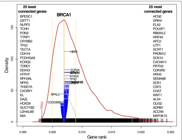
We start by computing GR and displaying the density along with the top least 25 and 25 top most connected genes out of 11,864; see Figure 3. These genes are displayed at left and right, respectively. For example, gene BPESC1 is the least connected while gene HCN2 is the most connected. The actual value of GR for each gene is depicted as a black vertical bar: BPESC1 corresponds to the leftmost bar and HCN2 corresponds to the right-most bar. The red curve depicts the density of the GR distribution with the Gaussian kernel using the bandwidth=0.00034. This value of the bandwidth, on one hand, reflects deviations in the distribution and, on the other hand, is not too bumpy. The blue cone-like part of the plot depicts the connection of a specific gene, in this particular example gene BCRA1, the most notable gene linked to breast and ovarian cancers, with remaining genes. This gene is the most typical gene in terms of its connectivity and it is mostly con-nected with gene NBR2. Indeed, this connection is well known from the literature [18], Suenet al.[19]. The width of the bar is proportional to the gene’s correlation coefficient with remaining genes. If the correlation is positive the bar extends to the right, other-wise to the left. Dotted lines on both sides correspond to 1 and−1 to facilitate judgment about the strength of the correlation. Also we show the names of 10 positively and two the most negatively correlated genes. As follows from this plot, less correlated genes are at the
0.000 0.005 0.010 0.015 0.020 0.025
0 50 100 150 Gene rank De ns it y 25 least connected genes BPESC1 GSTT1 NLRP2 TCHH PON3 TYRP1 CRYBB2 TP53 TECTA CDH19 PCDHGA9 KCNG2 TDRD1 DDX43 HTR1F RPH3AL NPR3 THSD7A CXORF1 KL DAZL HOXD9 GUCY1B2 LDHAL6B MIA 25 most connected genes HCN2 GRIN1 ELA2 POU3F1 RBMXL2 HNF4A APC2 UTF1 SCRT1 PRDM12 SOX10 CACNA1I PRTN3 CDK5R2 HRH3 SEMA6B SOX1 CSF3 CHAT WNT1 ALX4 OLIG2 ADRB1 ACCN4 MAP3K10 TP5 3 BRCA1 CENPF TMEM118 TIMELESS TPX2 ATAD5 SPAG5CITNCAPHTOP2A
NBR2
NPAL2
CCDC85B
bottom and more correlated genes are at the top (the yellow curve represents the density of the squared correlation distribution). Two important observations can be drawn from this plot: (1) the GR distribution is not normal and several components can be seen, as either bumps or changes in the density curvature, (2) among 11,863 genes only a handful of genes are highly correlated with BCRA1 (they are located in the top half of the blue plot), and the majority of the those genes are positively correlated.
Several the least connected genes are mentioned in the literature in association with ovarian cancer: The most prominent is TP3 (P53) which mutations lead to various types of cancer as reported in Schuijer and Berns [20]. It was documented by Gateset al.[21] that gene GSTT1 produces enzymes which catalyze carcinogens and increase the chance of the ovarian cancer; gene KL is associated with several types of cancer such as breast and lung, besides ovarian cancer; HTR1F is named among genes associated with ovarian cancer, see Codyet al.[22].
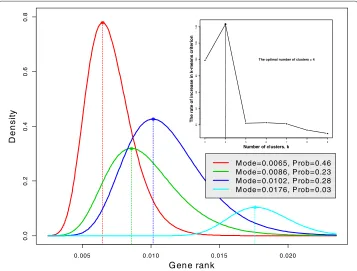
Now we draw our attention to the GR distribution. Visual inspection of the GR den-sity (red curve) reveals a possibility of several clusters of gene connectivity; an obvious connectivity cluster is where gene PKD1 is located. As was mentioned above, there are four clusters/subtypes of ovarian cancer genes. To test this finding, we plot the rate of increase of the criterion in the k-means algorithm versusk to determine at what k it reaches its maximum, according to the method of the L-curve; see Hansenet al. [23] (inset in Figure 4). According to this analysis ovarian cancer genes form four clus-ters/subtypes. The question we pose is as follows: Do these clusters impose four clusters in the gene connectivity and how can we determine these clusters using GR? We use the
3 4 5 6 7 8 9
20
40
60
80
100
120
14
0
Number of clusters, k
Th
e
r
a
te o
f
incr
ease
in k
-m
e
a
n
s
c
ri
ter
ion
The optimal number of clusters = 4
0.005 0.010 0.015 0.020
0.
0
0
.2
0.4
0
.6
0
.8
Gene rank
De
n
s
it
y
M ode= 0.0065, P rob= 0.46 M ode= 0.0086, P rob= 0.23 M ode= 0.0102, P rob= 0.28 M ode= 0.0176, P rob= 0.03
Gaussian mixture distribution technique (Hastieet al.[24]) to express the density of the GR distribution,f(p), using four components:
f(p)= k
i=1
πiφ p;μi,σi2
, (4)
whereφ p;μi,σi2
denotes the Gaussian density with meanμi and varianceσi2 andπi represents the proportion of genes in theith component,πi = 1. Since the distribu-tion of GR is skewed and positive, the mixture distribudistribu-tion is plotted on the log scale and then transformed back to original values. The result of parameter estimation using the Expectation-Maximization (EM) algorithm (Murphy [25]) is presented graphically in Figure 4. Four clusters/subtypes correspond to four density components depicted with different color. The majority of the genes (the first subtype probability,π1=46%, red)
have the lowest connectivity with mode=0.0065; the second and third subtypes (green and blue) have close connectivity with probability close to 25%. Genes from the fourth subtype are closely connected and they constitute the minority (probability,π4=3%).
Gene rank transformation during rice growth
The paper by Fujita et al. [26] examines how microarray gene expressions change dur-ing rice reproduction startdur-ing from pollination–fertilization and enddur-ing with zygote formation. The rice gene expression data comprise n = 57, 381 probes/genes and m = 99 samples; the data were obtained through the NCBI GEO DataSets website: http://www.ncbi.nlm.nih.gov/gds/. Rice, as well as other plants, goes through four stages of developmental progression: (1) anther development, (2) pollination–fertilization, (3) embryogenesis: the bottom quarter, and (4) embryogenesis: the top three quarters. We use GR to answer the following questions. Does the complexity of the gene network char-acterized by GR reflect the four transformations? If so, can one quantify the proportion of the gene network built at each stage? The assumption is that the correlation/connectivity between genes changes with the phenotype (in this case stage of the rice development progression). For validation purpose, we act in the reverse fashion: compute correlations using all data and see whether the distribution of GR reflects the four groups (the same approach is used for theDrosophiladata in the next section). A similar approach has been recently used by Langfelderet al.[27].
The result of our analysis is presented in Figure 5, where the gene rank, as the left maximum 57,381-dimensional eigenvector of matrixH, is computed using the algorithm outlined in Theorem/method 3 of the Appendix. The first two algorithms of GR com-putation do not work due to the large number of genes; it took eight iterations or about 3 minutes to achieve the accuracy of 10−5 on my desktop PC. The GR distribution on
0 20 40 60 80 100
0
.0
0
0
0
.0
05
0.
01
0
0
.0
1
5
0.
02
0
Gene rank, %
Dens
it
y
Gaussian kernel density Total density Anther development Pollination-fertilization
Embryogenesis: the bottom quarter Embryogenesis: the top three quarters
Figure 5 Identification of four developmental stages of rice using gene rank computed using algorithm described in Theorem 3 of the Appendix.The Gaussian mixture EM algorithm was used to estimate the components of the GR density.
these four rice transformations. Remarkably, the gene rank distribution estimates approx-imately equal (the proportion is about 25%) what was know from the pre-microarray biology of the plant. The fact that SDs at embryogenesis stage are larger may be explained by the fact that at the last stages of development the gene connections are more compli-cated compared with the early development and therefore more heterogeneous. However, further investigation is required to fully comprehend the insights from the gene rank results.
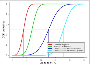
It seems obvious that later rice genome development should increase the complexity of the gene network. Can this statement be supported by our GR distribution at each stage? We use the cumulative distribution function (cdf ) to answer this question.
Definition 2. Let X and Y be two random variables. We say that X is smaller than Y in stochastic sense ifPr(X ≤ z) ≥ Pr(Y ≤ z),or in terms of the cumulative distribution function FX(z)≥FY(z),for every real z.
Table 1 Gaussian mixture GR distribution of rice growth
Developmental stage Mean SD Prop
μ σ π
Anther development 15.9 4.97 0.203
Pollination–fertilization 27.5 6.32 0.252
Embryogenesis: the bottom quarter 50.6 11.8 0.311
This definition can be interpreted as follows: For everyz, the proportion ofXvalues smaller thanz is larger than the proportion of Y values smaller than z. For example, using this definition, we can state that women are shorter than men in a stochastic sense because the proportion of women is larger than the proportion of men among people of height≤zfor eachz. Note that the inequality between the means does not imply stochas-tic inequality; however, it can be proven mathemastochas-tically that stochasstochas-tic inequality implies inequality between means and medians. The stochastic inequality is the most stringent inequality between random variables. We use this definition to demonstrate that the com-plexity (connectivity) of genes during rice development increases using the Gaussian cdf GR mixture distribution with parameters shown in Table 1; the results are presented in Figure 6. Indeed, the GR cdf for each consecutive stage shifts to the right indicating that “Embryogenesis: the top three quarters” has the highest and “Anther development” has the lowest gene rank. For example, we may consider the medians of GR for each rice development stage (depicted by thin lines with the appropriate color): While the median GR in the earliest stage is about 15%, the median GR in the latest stage is about 70%.
Comparison of gene rank across Drosophila organs
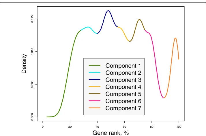
In this example, we demonstrate that gene connectivity changes from organ to organ in the same organism. We illustrate this phenomenon using the microarray data on Drosophila melanogaster (Chintapalliet al.[28]), which combines eight organs, brain, head, midgut, tubule, hindgut, ovary, testis, and accessory gland. Our hypothesis is that different organs exhibit different gene connectivities. To test this hypothesis, we compute GR using all samples to see whether its density reflects a multi component
0 20 40 60 80 100
0
.0
0
.20
.40
.6
0
.81
.0
G ene rank, %
C
D
F
, pr
obabi
lit
y
Anther development Pollination-fertilization
Embryogenesis: the bottom quarter Embryogenesis: the top three quarters
character. Indeed, as follows from Figure 7, the distribution of gene rank is multimodal and represents seven clusters of values attributable to different fly organs.
Comparison of the gene rank across organisms
The gene network connectivity/complexity should increase from simple to complex organisms. While everybody agrees with this statement, there is no rigorous empirical verification of this conjecture. We tackle this question using microarray data from the three experiments, rice,DrosophilaandHomo sapiens, analyzed previously, by plotting the empirical GR cdfs on the same graph; see Figure 8. Following definition of stochas-tic inequality, rice has the smallest gene connectivity andHomo sapienshas the largest connectivity (the median GR is where the cdf=0.5). Remarkably, there exists a strong separation between the three organisms despite the fact that gene expressions represent different organs at different stages of development.
Conclusions
We have introduced a new concept that reflects gene connectivity, the gene rank (GR). GR augments oura priori knowledge about gene connection using microarray experiment data. We have shown by examples that the new measure reflects biological expectations and may lead to insights of gene network development in time, across organs of the same organism and across organisms. GR may be used for hypothesis generation in establish-ment of gene pathways. For example, the fact that many least connected genes are among genes directly associated with ovarian cancer is illuminating.
Traditional gene ranking based on thet-test or, in general, based on correlation with a phenotype and our GR look at the microarray data matrix orthogonally. The pheno-type approach uses the horizontal correlation of genes with phenopheno-type. In contrast, GR reflects the vertical correlation across genes, so the phenotype information is not used.
0 20 40 60 80 100
0
.000
0
.0
0
5
0.
010
0.
0
15
Gene rank, %
De
n
s
ity
Component 1 Component 2 Component 3 Component 4 Component 5 Component 6 Component 7
0.000 0.005 0.010 0.015 0.020
0
.00
.2
0
.40
.60
.81
.0
G ene rank
C
D
F,
probabi
lit
y
H om o sapiens
D rosophila
R ice
Figure 8 Comparison of gene connectivity across three organisms using cdf.The higher the cdf, the more connected are the genes.
Both angles of microarray data analysis are important and valid. However, we believe that GR is more fundamental from the biological point of view, although the t-test may be more clinically important.
We have shown that GR can be used for identification of gene hubs (Choi and Kendziorski [29], Wuet al.[30]) as an alternative to cluster analysis. This cross-gene mea-sure can be used to modify thet-test and the respective threshold for thep-value to reduce the false discovery rate in genome-wide association studies; see Zuber and Strimmer [4], Yassouridis [31].
In this work, a simple constant a priori assumption (constant damping factor) was used for gene connectivity. More work must be done to enrich the GR computation with available gene network connection information such as GO or IMP (Wonget al.[32]). For example, ifAijis a binary connectivity matrix build on the basis of GO annotations (Aij=1 if genesiandjare connected and 0 otherwise, assuming thatAii=1) we may set aj=1−ni=1Aij/ni=1
n
j=1Aij. Use ofa prioribiological information may leverage the possibility of false correlation especially important in the case of a small sample size,m.
We have presented just a small amount of empirical evidence that GR can be used to characterize the complexity of genes’ connections in organs and organisms. More studies are required to understand its usefulness as a characteristic of genetic complexity.
Appendix
Proof that matrixHis a stochastic matrix
matrix language thatH1=1. First, we observe thatR2∗1=1since the sum of elements in each row of matrixR2∗is 1. Second, since11=nandA1=a, we have
H1 =
1
n(1−a)1
+AR2
∗
1=1
n(1−a)1
1+AR2
∗1
= 1
n(1−a)n+A1=(1−a)+a=1,
matrixHis a stochastic matrix and, therefore, the Perron-Frobenius theorem applies.
Computation of the left maximum eigenvector
Below we describe three methods for computation of GR under three assumptions regarding the size of the microarray matrix. In all computations the noninformative prior on gene connectivity is used with constanta=0.9. In case of an informative prior, vector
ashould specify connectivity between 0 and 1.
1. Using the built-in function eigen in R for smalln. When the number of genes is fairly small, say,n < 5000 computation of the left maximum eigenvector can be done using a built-in function in various software packages. For example, inRthis function is
eigen.
a=0.9
n=nrow(X)
R2=cor(X)^2
one.n=rep(1,n)
sum.row=R2%*%one.n R2.star=(1/sum.row)*R2 H=(1-a)/n+a*R2.star
p=abs(eigen(t(H))$vectors[,1])
Note that ifpis an eigenvector−pis an eigenvector. too. Therefore, we take the absolute value of the eigenvector ofHin the last line.
2. The power method for moderaten, say, 5000< n< 10000. It is well known that the left maximum eigenvector with the unit eigenvalue can be computed iteratively as
pk+1=Hpk, k=0, 1,. . .
This method is referred to as the power method [33]. The followingRcode realizes this method starting fromp0=R21/R21. As in the previous method we seta=0.9;eps
andmaxitspecify the convergence tolerance and the maximum number of iterations.
eps=0.0001;maxit=10
a=0.9
n=nrow(X)
R2=cor(X)^2
one.n=rep(1,n)
p=sum.row/sqrt(sum(sum.row^2))
for(it in 1:maxit)
{
p.new=tH%*%p
p.new=p.new/sqrt(sum(p.new^2))
adiff=max(abs(p-p.new))
if(adiff<eps) break
p=p.new
}
return(p.new)
Typically, this algorithm requires less than 10 iterations to converge. Moreover, for fairly largen, say,n>1000 it may be even faster and more precise then using theeigen func-tion becauseeigencomputes all eigenvalues and eigenvectors, but the power method computes only the maximum eigenvector.
3. Computation of the gene rank for largen, say,n > 10000. As in many datasets, even computation of an 50000×50000 correlation matrix using the built-in functioncor
becomes troublesome ( Rreports an error due to lack of memory). Below, we suggest an algorithm based on the power method without computation of the correlation matrix. This algorithm is especially effective whennis large andmis relatively small, say,m < 500. For example, it took 3 minutes to compute GR for the rice data usint R version 3.0.1 on myAcerlaptop (Windows 7, 64 bit, 4 GB RAM, processor Intel(R) CPU @ 1.60 GHz). In order to avoid computation of a large-sizeR2, we need to compute the normalized gene expression matrix X, by subtracting the mean over samples and dividing by the norm. Specifically, compute
zi=
xi−xi1m xi−xi1m
, (5)
so that the rows of then×mmatrixZarezi. Importantly, computation of the normalized matrix, Zmay be accomplished in a vectorized fashion inRwith no loop and therefore very efficiently, as shown below.
x.bar=rowMeans(X)
Xsub.mean=X-x.bar
sdX=sqrt(rowSums(Xsub.mean^2))
Z=(1/sdX)*Xsub.mean
Then, obviously,R = ZZ. In the theorem below, we expressR21and more generally (R2∗)pwithout computation ofR2. The formulas require a double loop overm, but for smallm, it is more efficient than computation of a largeR2.
Theorem 1.Let the n×n correlation matrix be expressed asR= ZZandR2be the squared correlation matrix. Then the following representation holds
R21=
m
k=1
m
l=1
where
gkl =Z·kZ·l, vkl=Z·kZ·l,
Z·kandZ·lare the k th and the l th columns of the normalized matrix,Z, andrepresents the element-wise vector or matrix multiplication. Further, ifpis any n×1 vector, the following representation holds.
R2∗p=
m
k=1
m
l=1
hklvkl (7)
where
hkl=Z·k
Z·l
p R21
. Proof. Represent R= m
k=1 Z·kZ·k.
This implies
R2=
m
k=1
m
l=1 Z·kZ·k
Z·lZ·l
.
Now we use the formula(ab)(cd)=(ac)(bd), wherea,b,c,dare vectors [34]. This leads to the representation
R2=
m
k=1
m
l=1
(Z·kZ·l)(Z·kZ·l).
so that
R21=
m
k=1
m
l=1
(Z·kZ·l)(Z·kZ·l)1
But(Z·kZ·l)1=Z·kZ·l =gklleading to formula (6). To prove formula (7), we rewrite
(R2∗)p=R2p∗, where p∗ = p/(R21) assuming the element-wise division, and R21is defined by (6). But
R2p∗=
m
k=1
m
l=1
(Z·kZ·l)(Z·kZ·l)p∗
finally leading to formula (7). The theorem is proved.
Below, we show theRcode that implements this algorithm.
eps=0.0001;maxit=10
a=0.9
sumR2=rep(0,n)
for(i in 1:m)
for(j in 1:m)
{
qij=sum(Z[,i]*Z[,j])
p=sumR2/sqrt(sum(sumR2^2))
for(it in 1:maxit)
{
tR2p.fast=rep(0,n)
for(i in 1:m)
for(j in 1:m)
{
hij=sum(Z[,i]*Z[,j]*p/sumR2)
tR2p.fast=tR2p.fast+hij*Z[,i]*Z[,j] }
p.new=(1-a)/n*sum(p)+a*tR2p.fast p.new=p.new/sqrt(sum(p.new^2))
adiff=max(abs(p-p.new))
if(adiff<eps) break
p=p.new
}
Competing interests
The author declares that he has no competing interests.
Acknowledgments
I thank my colleagues at Dartmouth, Drs. Jennifer Doherty and Scott Williams, who read a draft of the manuscript and made useful comments and suggestions, and Jason Moore for his support. Also I am thankful to Brett McKinney, the reviewer for his comments and constructive criticism. This work was supported by the NIH grants P20RR024475 and P20GM103534.
Received: 21 June 2014 Accepted: 4 December 2014
References
1. Page L, Brin S, Motwani R, Winograd T. The PageRank citation ranking: bringing order to the web, Technical report, Stanford Digital Library Technologies Project 1998. http://ilpubs.stanford.edu:8090/422/1/1999-66.pdf.
2. Morrison JL, Breitling R, Higham DJ, Gilbert DR. GeneRank: Using search-engine technology for the analysis of microarray experiments. BMC Bioinformatics. 2005;6:233–46.
3. Winter C, Kristiansen G, Kersting S, Roy J, AustD, Knösel T, Rümmele P, et al. Google goes cancer: Improving outcome prediction for cancer patients by network-based ranking of marker genes. PLOS Comput Biol. 2012;8: e1002511.
4. Zuber V, Strimmer K. Gene ranking and biomarker discovery under correlation. Bioinformatics 2009;25:2700–7. 5. Opgen-Rhein R, Strimmer K. Accurate ranking of differentially expressed genes by a distribution-free shrinkage
approach. Stat Appl Genet Mol Biol. 2007;6:9.
6. Nitsch D, Goncalves JP, Ojeda F, de Moor B, Moreau Y. Candidate gene prioritization by network analysis of differential expression using machine learning approaches. BMC Bioinformatics. 2010;11:460.
7. Masoudi-Nejad A, Meshkin A, Haji-Eghrari B, Bidkhori G. Candidate gene prioritization. Mol Genet Genomics. 2012;287:679–98.
8. Langfelder P, Horvath S. WGCNA: an R package for weighted correlation network analysis. BMC Bioinformatics. 2008;9:559.
9. Gelman A, Carlin JB, Stern HS, Dunson DB. Bayesian Data Analysis, 3rd ed. Boca Raton: Chapman & Hall; 2013. 10. Berman A, Plemmons RG. Nonnegative matrices in the mathematical sciences. PA: SIAM Philadelphia; 1994. 11. Golub GH, Greif C. An Arnoldi-type algorithm for computing page rank. BIT Numer Math. 2006;46:759–71. 12. Wu G, Xu W, Wei Y. A preconditioned conjugate gradient algorithm for GeneRank with application to microarray
data mining. Data Mining Knowl Discov. 2013;26:27–56.
13. R Development Core Team. A language and environment for statistical computing. Vienna, Austria: R Foundation for Statistical Computing; 2012. ISBN 3-900051-07-0, URL http://www.R-project.org/.
14. Rosenwald A, Wright G, Chan WC, Connors JM, Campo E, Fisher RI, Gascoyne RD, Muller-Hermelink HK, Smeland EB, Staudt LM. The use of molecular profiling to predict survival after chemotherapy for diffuse large-B-cell lymphoma. N Engl J Med. 2002;346:1937–1947.
15. The Cancer Genome Atlas Research Network. Integrated genomic analyses of ovarian carcinoma. Nature. 2011;474: 609–15.
16. The cancer genome atlas completes detailed ovarian cancer analysis 2013. http://www.cancer.gov/newscenter/ newsfromnci/2011/TCGAovarianNature.
18. NBR2 neighbor of BRCA1 gene 2 (non-protein coding) [Homo sapiens (human). http://www.ncbi.nlm.nih.gov/gene/ 10230.
19. Suen TC, Tang MS, Goss PE. Model of transcriptional regulation of the BRCA1-NBR2 bidirectional transcriptional unit. Biochim Biophys Acta. 2005;1728:126–34.
20. Schuijer M, Berns EMJ. TP53 and ovarian cancer. Hum Mutat. 2003;21:285–91.
21. Gates MA, Tworoger SS, Terry KL, Titus-Ernstoff L, Rosner B, De Vivo I, et al. Talc use, variants of the GSTM1, GSTT1, and NAT2 genes, and risk of epithelial ovarian cancer. Cancer Epidemiol Biomarkers Prev. 2008;17:2436–44. 22. Cody NAL, Shen Z, Ripeau JS, Provencher DM, Mes-Masson AM, Chevrette M, et al. Characterization of the
3p12.3-pcen region associated with tumor suppression in a novel ovarian cancer cell line model genetically modified by chromosome 3 fragment transfer. Mol Carcinog. 2009;48:1077–1092.
23. Hansen PC. Analysis of the discrete ill-posed problems by means of the L-curve. SIAM Rev. 1992;34:561–580. 24. Hastie T, Tibshirani R, Friedman J. The Elements of Statistical Learning, 2nd ed. New York: Springer; 2009. 25. Murphy KP. Machine learning. a probabilistic perspective. Cambridge, MA: The MIT Press; 2012.
26. Fujita M, Horiuchi Y, Ueda Y, Mizuta Y, Kubo T, Yano K, et al. Rice expression atlas in reproductive development. Plants Cell Physiol. 2010;51:2060–81.
27. Langfelder P, Mischel P, Horvath S. When is hub gene selection better than standard meta-analysis. Plos One. 2013;e61505:8.
28. Chintapalli VR, Wang J, Dow JAT. Using FlyAtlas to identify better. Drosophila melanogaster models of human disease. Nat Genet. 2007;39:715–20.
29. Choi Y, Kendziorski C. Statistical methods for gene set co-expression analysis. Bioinformatics 2009;25:2780–86. 30. Wu XG, Huang H, Sonachalam M, Reinhard S, Shen J, Pandey R, et al. Reordering based integrative expression
profiling for microarray classification. BMC Bioinformatics. 2012;13(Suppl. 2):article S1.
31. Yassouridis A, Ludwig T, Steiger A, Leisch F. A new way of identifying biomarkers in biomedical basic-research studies. PLOS ONE. 2012;e35741:7.
32. Wong AK, Park CY, Greene CS, Bongo LA, Guan YF, Troyanskaya OG. IMP: A multi-species functional genomics portal for integration, visualization and prediction of protein functions and networks. Nucleic Acids Res. 2012;40:W484–90. 33. Golub GH, Van Loan CF. Matrix Computations, 3d ed. Baltimore: Johns Hopkins University Press; 1996.
34. Schott JR. Matrix Analysis for Statistics, 2nd ed. New York: Wiley; 2005.
Submit your next manuscript to BioMed Central and take full advantage of:
• Convenient online submission
• Thorough peer review
• No space constraints or color figure charges
• Immediate publication on acceptance
• Inclusion in PubMed, CAS, Scopus and Google Scholar
• Research which is freely available for redistribution