www.the-cryosphere.net/7/1659/2013/ doi:10.5194/tc-7-1659-2013
© Author(s) 2013. CC Attribution 3.0 License.
The Cryosphere
Parameter and state estimation with a time-dependent adjoint
marine ice sheet model
D. N. Goldberg and P. Heimbach
Earth, Atmospheric and Planetary Sciences, M.I.T., Cambridge, USA. Correspondence to: D. N. Goldberg ([email protected])
Received: 16 May 2013 – Published in The Cryosphere Discuss.: 17 June 2013
Revised: 30 September 2013 – Accepted: 10 October 2013 – Published: 6 November 2013
Abstract. To date, assimilation of observations into
large-scale ice models has consisted predominantly of time-independent inversions of surface velocities for basal trac-tion, bed elevatrac-tion, or ice stiffness, and has relied primarily on analytically derived adjoints of glaciological stress bal-ance models. To overcome limitations of such “snapshot” in-versions – i.e., their inability to assimilate time-dependent data for the purpose of constraining transient flow states, or to produce initial states with minimum artificial drift and suitable for time-dependent simulations – we have devel-oped an adjoint of a time-dependent parallel glaciological flow model. The model implements a hybrid shallow shelf– shallow ice stress balance, solves the continuity equation for ice thickness evolution, and can represent the floating, fast-sliding, and frozen bed regimes of a marine ice sheet. The adjoint is generated by a combination of analytic meth-ods and the use of algorithmic differentiation (AD) software. Several experiments are carried out with idealized geome-tries and synthetic observations, including inversion of time-dependent surface elevations for past thicknesses, and simul-taneous retrieval of basal traction and topography from sur-face data. Flexible generation of the adjoint for a range of independent uncertain variables is exemplified through sen-sitivity calculations of grounded ice volume to changes in basal melting of floating and basal sliding of grounded ice. The results are encouraging and suggest the feasibility, using real observations, of improved ice sheet state estimation and comprehensive transient sensitivity assessments.
1 Introduction
Simulation of land ice evolution is hampered by a great num-ber of sources of uncertainties regarding poorly or unknown quantities which exert control over ice dynamics. These un-certainties must be dealt with to address questions regard-ing the estimation of past ice flow and future behavior of ice sheets and glaciers. Unknown quantities often take the form of spatial fields rather than scalars, requiring computational techniques that can handle sets of unknowns which scale with model dimension, but with computational costs largely inde-pendent of that dimension. The adjoint or Lagrange multi-plier method is an ideal candidate.
The adjoint of a (generally nonlinear) model is essen-tially the transpose of its Jacobian, the Jacobian being the linear map of perturbations to model input (e.g., its initial and boundary conditions) to perturbations in output, for a given model realization. Assuming the model is differen-tiable, the Jacobian can, in principle, be estimated with fi-nite differences. However, when the size of the parameter set numbers in the thousands or millions, as is the case in land ice models, such an approach quickly becomes intractable. With the adjoint method, on the other hand, gradient or sen-sitivity information of the model output with respect to its input is obtained efficiently. Its computational cost is inde-pendent of the size of the input set, making gradient-based optimization/estimation for large-scale problems with high-dimensional input spaces tractable.
almost exclusively to estimate basal or interior properties of ice sheets and ice shelves (e.g., basal traction param-eters, stiffness parameters) based on observations of sur-face velocities. The first such application was by MacAyeal (1992), who used a depth-integrated stress balance (Morland, 1987; MacAyeal, 1989). In recent years, similar inversions have been carried out with so-called “higher-order” mod-els, i.e., models that incorporate vertical inhomogeneity and even nonhydrostatic effects (e.g., Maxwell et al., 2008; Ray-mond and Gudmundsson, 2009; Goldberg and Sergienko, 2011; Morlighem et al., 2010; Arthern and Gudmundsson, 2010; Gillet-Chaulet et al., 2012; Petra et al., 2012). How-ever, all these inversions consider only the nonlinear stress balance; i.e., they do not take the time-dependent mass bal-ance into account. Furthermore, they only consider uncer-tainties in surface velocities (not, for instance, in surface ele-vation or thickness). Brinkerhoff et al. (2011) applied an ad-joint method to a flowline Stokes model coupled to a steady-state thermal balance, but there was no time dependence in the model. An example of the use of a time-dependent ice model is that of Heimbach and Bugnion (2009), in which the adjoint of SICOPOLIS (Greve, 1997), a thermo-mechanical ice model which makes the shallow ice approximation (SIA; Hutter, 1983), was generated.
A natural extension to the work of Heimbach and Bugnion, then, is the application of adjoint methods to time-dependent ice models that include horizontal stress coupling in the non-linear momentum balance. Such an approach has the advan-tage that the prognostic components of the ice model, such as thickness and temperature evolution, are accounted for in the model adjoint, thus enabling assimilation of time-dependent data to produce a dynamically consistent state estimate with associated optimized parameters. In the field of ocean model-ing, state estimation efforts based on the adjoint method were first introduced by Thacker and Long (1988) and Tziper-man and Thacker (1989). Since then, estimation systems, in which the adjoint was derived by means of automated dif-ferentiation of full-fledged ocean general circulation mod-els, have provided solutions that are consistent with obser-vational data, suitable for model initializations and in-depth data analysis, as well as a framework for estimating the in-formation content of new observations (Stammer et al., 2002; Wunsch et al., 2009; Wunsch and Heimbach, 2013). While ice sheet state estimation is still in its infancy, we view ocean state estimation as a model paradigm, and time-dependent ice model adjoints as a step toward this goal.
In this paper, we present the adjoint generation of a time-dependent ice sheet–stream–shelf model. The ice model im-plements a “hybrid” stress balance (e.g., Bueler and Brown, 2009; Pollard and DeConto, 2009; Schoof and Hindmarsh, 2010; Goldberg, 2011), which is the simplest form of higher-order stress balance, yet still it accounts for horizontal stress coupling, which makes our approach novel. Prior to this study, the adjoint method has not been applied to a time-dependent ice model with a nonlocal stress balance.
Ray-mond and Gudmundsson (2009) developed a method for a maximum a posteriori (MAP) estimate of basal properties in terms of observed surface properties, taking the steady state of the continuity equation into account. Their forward model contains the full Stokes stress balance without approxima-tion. However, it is in a single horizontal dimension, and is based on analytical transfer functions that assume Newtonian rheology as well as small perturbations about a mean state (Gudmundsson, 2003). In addition to the conceptual novelty of using a time-evolving adjoint model for inversion, a tech-nical novelty of our study is the use of algorithmic (or au-tomatic) differentiation (AD) (Griewank and Walther, 2008) for an ice model that involves longitudinal (nonlocal) stress balance terms. AD tools are a powerful array of software that are capable of generating adjoint model source code via line-by-line differentiation of the numerical model. The pliability of the AD tools means that sensitivities to diverse sets of in-puts can be examined, and changes to the input set, the cost function, and the forward model can be reflected in the ad-joint much more easily than through separate error-prone by-hand adjoint code extensions. Finally, the approach provides the exact adjoint of the discrete model. In some of the glacio-logical studies mentioned above, the nonlinear dependence of viscosity on strain rates has been ignored in the adjoint calculation. which is generally a safe approximation, but in some cases has been shown to cause difficulties with model inversion (Goldberg and Sergienko, 2011).
The ice sheet stress balance equations (depth-integrated or otherwise) have a differentiable structure which consid-erably simplifies the derivation of their adjoint. This, and the fact that they do not involve time stepping, enables straight-forward discretization of the adjoint differential equations. This option is, in practice, much simpler than applying AD, which is not well-suited to iterative methods, such as those used to solve the nonlinear elliptic partial differential equa-tions of the ice models. On the other hand, other conservation equations involved in solving the ice flow, such as the thick-ness (or continuity) equation or conservation of heat, only solve for local interdependencies and are well suited for AD. The adjoint of Heimbach and Bugnion, as well, was gener-ated with AD tools – the only instance of AD application to a land ice model. Here, we shall adopt a mix-and-match strategy, using both AD-generated code and “hand-written” solvers where this appears more efficient to produce the exact model adjoint.
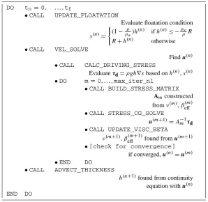
Table 1. Pseudocode version of forward model time-stepping procedure.
DO tn=0, . . . ,tf
•CALL UPDATE_FLOATATION
Evaluate floatation condition
s(n)=
( (1− ρ
ρw)h
(n) ifh(n)≤ −ρw
ρ R
R+h(n) otherwise
•CALL VEL_SOLVE
Findu(n)
•CALL CALC_DRIVING_STRESS
Evaluateτd=ρgh∇sbased onh(n),s(n)
•DO m=0, . . . ,max_iter_nl
•CALL BUILD_STRESS_MATRIX
Amconstructed fromν(m),βeff(m)
•CALL STRESS_CG_SOLVE
u(m+1)=A−m1τd
•CALL UPDATE_VISC_BETA
ν(m+1),βeff(m+1)found fromu(m+1)
•[check for convergence]
if converged,u(n)=u(m)
•END DO
•CALL ADVECT_THICKNESS
h(n+1)found from continuity equation withu(n)
END DO
2 Forward model
The ice model used in this study is an extension of the stress balance solution presented in Goldberg (2011). It is a hybrid model, also referred to as L1L2 under the Hindmarsh (2004) classification, meaning it accounts for vertical shear in its stress balance, although not as completely as the Blatter– Pattyn balance (Blatter, 1995; Pattyn, 2003; Greve and Blat-ter, 2009). On the other hand, the balance requires the solu-tion of a two- rather than three-dimensional nonlinear ellip-tic differential equation, greatly reducing computational ex-pense. The balance is derived by making an approximation to the variational principle corresponding to the Blatter–Pattyn equations rather than to the equations themselves. It has been demonstrated to be a good approximation to Blatter–Pattyn and to Stokes flow (Sergienko, 2012), especially when some level of basal sliding is present. In addition, the model solves the depth-integrated continuity equation for ice thickness and accounts for grounded and floating ice through a hydrostatic floatation condition.
Table 1 is a pseudocode version of the ice model. We present this diagram for clarity, but also in order to aid the description of adjoint generation in the following section. At the beginning of a given time step,h(n), the thickness at time tnis known. The cells that are floating are determined from the hydrostatic floatation condition:
h(n)≤ −ρw
ρ R, (1)
whereρwandρare ocean and ice densities, respectively, and Ris bed elevation (negative when below zero). This also de-termines surface elevations(n), because when the ice is float-ing a fraction (ρρ
w)of total column thickness is below sea
level. These operations are represented in the pseudocode by
UPDATE_FLOATATION, which also sets the contribution of basal sliding coefficients to zero in floating cells.
Following this call the nonlinear hybrid stress bal-ance is solved for velocity u(n), using the scheme from Goldberg (2011). This involves first evaluating the dis-cretized form of the glaciological driving stressτd=ρgh∇s (CALC_DRIVING_STRESS), which depends on s(n) and h(n). This is then followed by Picard iteration on viscos-ity and basal coefficients. In each iteration m of the loop, the matrixAm(corresponding to the two-dimensional ellip-tic PDE mentioned above) is constructed, using current iter-ates of nonlinear ice viscosityν(m)and basal coefficientβeff(m) (BUILD_STRESS_MATRIX).
βeff is a variable unique to the stress balance derived in Goldberg (2011), and thus its form is given here for the ben-efit of the reader:
βeff=
f (ub)
ub
1+ωf (ub)
hub
. (2)
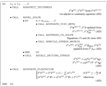
Table 2. Pseudocode version of adjoint model reverse-time-stepping algorithm corresponding to Table 1. (AD) indicates that this step is processed by the algorithmic differentiation tools.
DO tn=tf, . . . ,0
•CALL ADADVECT_THICKNESS
δ∗u(n),δ∗h(n)fromδ∗h(n+1)
via adjoint to continuity equation (AD)
•CALL ADVEL_SOLVE
•DO m=mterm, . . . ,0
•CALL ADUPDATE_VISC_BETA
δ∗u(m+1),δ∗βupdated from
δ∗ν(m+1),δ∗βeff(m+1)(AD)
•CALL ADSTRESS_CG_SOLVE
Equations (7) and (8) (non-AD)
•CALL ADBUILD_STRESS_MATRIX
δ∗ν(m),δ∗βeff(m),δ∗Bglen,δ∗h(n) updated fromδ∗Am(AD)
•END DO
•CALL ADCALC_DRIVING_STRESS
δ∗h(n)=ρg∇s(n)(δ∗τd),
δ∗s(n)=ρgh(n)(∇ ·δ∗τd)
(AD)
•CALL ADUPDATE_FLOATATION
(
δ∗h(n)=δ∗h(n)+(1− ρ
ρw)δ
∗s(n) ifh(n)≤ −ρw
ρ R
(δ∗h(n), δ∗R)=(δ∗h(n), δ∗R)+δ∗s(n) otherwise (AD)
END DO
stress (τb) and sliding velocity:
τb= f (ub)
ub
u|z=b. (3)
ub is determined from basal stress and depth-averaged ve-locity under the approximation of depth-independent longi-tudinal stresses, andωis a factor that depends on the current iterate of viscosity, as defined in Goldberg (2011) (Eq. 35).
Next the resulting linear systemAmu(m+1)=τdis solved for the new iterate ofu(STRESS_CG_SOLVE). The non-linear ice viscosity and sliding coefficients are then updated with this new guess for velocity (UPDATE_VISC_BETA).
Following the velocity solve, thickness is updated via the depth-integrated continuity equation, using a simple second-order flux-limited finite volume scheme. If calving front ad-vance is allowed, this is carried out using an algorithm based on that of Albrecht et al. (2010), though no calving param-eterization has been implemented. This all takes place in
ADVECT_THICKNESS, and concludes the time step. In the hybrid balance, the viscosityν and sliding coeffi-cientβeff(which depends on velocity even for a linear slid-ing law) have slightly more complicated expressions than in the SSA balance. However, under the Picard iterative scheme employed, the updates of these fields are straightforward. Additionally,UPDATE_VISC_BETAcan seamlessly be
re-placed by an SSA viscosity update, effectively making the model a shallow-shelf model.
a future development direction. However, the most important benefit for present purposes is that we are able to take advan-tage of the adjoint generation framework within the MITgcm, as discussed in the following section.
3 Model adjoint
The notion of “adjoint” is best understood in terms of its con-struction. Assume that, in a time-dependent ice model, one were concerned with how the initial thickness at a single lo-cation affected the thickness field at the end of the run. As-sume the initial thickness field is represented by a vectorh(0), and the thickness at the final time steptnbyh(n). If the model is differentiable, one can then consider a perturbation to a sin-gle element ofh(0) (i.e., a directional derivative) and propa-gate the perturbation forward to the final time to the resulting perturbation in the model output. This forward-propagation of perturbations is known as a tangent linear model (TLM). The TLM provides information about sensitivities of model output to a single variable (i.e.,h(0)(i), the value ofh(0) in celli). If one wanted information about sensitivities to all suchh(0)k ,k=1, ..., M, whereMis the size of the grid, the TLM would need to be runMtimes. (Note that in this con-text, the “single location” referred to above is not a point in space, but rather a localized area that depends on the model’s discrete representation of a continuous field. If the represen-tation were spectral in nature, a localized value could not be well represented by a single degree of freedom.)
On the other hand, the adjoint can provide this informa-tion in a single run, provided the output of interest is scalar-valued. This scalar is often referred to as a cost, objective, or target function, for instance, the total volume of ice in the domain at the end of the run. The adjoint model is referred to as such because it is the mathematical adjoint of the TLM. This seemingly trivial distinction has important implications for how the models are constructed. For the TLM, the for-ward perturbation is found by successive compositions of the TLMs of sequential time steps. The adjoint model operates backwards in time, by composing the adjoints of individual time steps (or operations within time steps) in reverse order. The eventual result of the TLM is the sensitivity of the out-put to a single inout-put variable, whereas the result of the adjoint model is the sensitivity of a single scalar output to a set of in-put variables. In the remainder of this section we give an out-line of the generation of our ice model adjoint, highlighting the varied approaches employed. For a more comprehensive discussion of the mathematical meaning and implications of adjoint models, see Heimbach and Bugnion (2009).
First we introduce notation that will aid our discussion. Each state variable of the model has a corresponding vari-able in the adjoint model state (or more formally, a co-vector in the dual to the tangent space of the model at the given point in state space). For a state variablex, we denote its tangent space counterpart byδx, and its adjoint byδ∗x. In
gener-ating the adjoint we relate the adjoint state variables to one another. Assume the state variableyderives fromx through the atomic operationy=g(x). To generate the tangent linear model, we findδy, the perturbation toy, by applying the lin-ear operator∂g∂xtoδx. Conversely, we track sensitivities of a cost functionJfrom the final time backward. This means, if the sensitivities ofJtoyare stored inδ∗y, we findδ∗xby applying the adjoint of∂g∂xtoδ∗y.
In Table 3 we give a pseudocode version of the ad-joint ice model, corresponding to the version of the for-ward model presented in Table 1. The time-stepping loop is now from the final time tf to 0. Note that the inter-mediate steps of a single time step occur in reverse order, and the adjoint of the Picard iteration loop begins from
mterm, the termination step of the forward Picard loop.
From this it can be seen how initial condition sensitivi-ties, denotedδ∗h(0)≡ ∇[
h(0)]J, might be found, as well as
parameter sensitivities. For instance, βeff derives in part from the sliding parameter fieldβ in the pseudo-subroutine
UPDATE_VISC_BETA, and so contributions toδ∗βare cal-culated in ADUPDATE_VISC_BETA. Note that the diver-gence operator in ADCALC_DRIVING_STRESS is actu-ally the discrete divergence, corresponding exactly to the discretized gradient operator CALC_DRIVING_STRESS. Note also that the updates of δ∗h(n) and δ∗R from δ∗s(n) in ADUPDATE_FLOATATION involve the same condi-tional statement as in UPDATE_FLOATATION. Also in this pseudo-subroutine, the backward propagation of β -sensitivities are terminated where the floatation condition is satisfied.
matrix solve, is not handled by AD. The conjugate gradient algorithm employed involves a large number of intermediate variables relevant only to the solver, and can require many it-erations. A direct application of AD tools to the solver would involve large memory requirements, as well as a great deal of either code modification or manual “directing” of the tools, to prevent costly recomputation loops. On the other hand, TAF (as well as other AD tools) offers a facility to replace the adjoint code that is automatically generated by manually written code at the subroutine level, if the adjoint of a sub-routine is known, as is the case with the linear solver. As in Table 1, the linear solve can be written
u(m+1)=A−m1τd, (4) whereu(m+1)is the iterate of velocity found at stepmof the Picard loop,Amis the matrix constructed with the previous iterates of viscosity and basal coefficient, andτd is the driv-ing stressρgh∇sat the current time step. The solve can be viewed as an operatorgwith argumentsAmandτd, i.e.,
g:(Rn×n×Rn)→Rn; (5)
thus the adjoint operator must have the form
g∗:Rn→(Rn×n×Rn). (6)
The adjoint of Eq. (4) is given by δ∗τd=δ∗τd+A−mTδ
∗u(m+1), (7)
δ∗Am= −δ∗τd(u(m+1))T. (8)
Equation (7) is written as an accumulation of adjoint sen-sitivities ofτd; the adjoint of each Picard iteration has an effect onδ∗τd. In our adjoint model, a subroutine carries out these operations; sinceAmis self-adjoint, the same conjugate gradient solver (with the same matrix coefficients) is used in Eq. (7). Note that in the MITgcm ocean model, which solves a linear system for either rigid-lid surface pressure or free surface elevation, an equation similar to Eq. (7) is solved by the adjoint model, and the symmetry of the matrix is simi-larly exploited. However, the coefficients of the matrix are fixed, and so Eq. (8) has no counterpart. Following the so-lution of Eq. (7) and Eq. (8) by hand-written code, evalua-tion of the adjoint via AD-generated code is resumed:δ∗τd andδ∗Aiare passed to the adjoint of the matrix construction,
ADBUILD_STRESS_MATRIX.
An important by-product of this approach (“hiding” the matrix inversion from the AD software) is that it allows us to potentially replace our linear solver with faster, optimized “black-box” solvers (such as those available in external pack-ages such as PETSc) without affecting the accuracy of the adjoint. We point out that the advantages mentioned here are not limited to our model, i.e., to one that implements a shallow-shelf or hybrid stress balance. Matrix inversion is
the most time-intensive component of any ice model with a nonlocal stress balance, and the part of the code that is most likely to lead to difficulties in application of AD software. As long as it can be handled in a similar way to our model (i.e., as long as the matrix is self-adjoint), efforts can be fo-cused on ensuring that the remainder of the code is suitable for algorithmic differentiation.
It was found that, in order that the adjoint model produce accurate results, the CG tolerance for the linear solve in the adjoint needed to be several orders of magnitude smaller than that used in the linear solve of the forward model. (The ac-curacy is assessed by comparing the derivatives calculated by the adjoint to finite-difference approximations. Relative agreement to within 10−6 was considered accurate.) This suggests that without special treatment of the convergence criteria, a fully AD-generated adjoint might have low accu-racy, and further supports our decision to let the AD software “bypass” our linear solver.
4 Nonlinear optimization
For optimization problems, our model uses the M1QN3 li-brary, publicly available Fortran code which is based on the algorithm described in Gilbert and Lemaréchal (1989). The M1QN3 algorithm solves large-scale unconstrained mini-mization problems. It provides a search direction and step size based on a limited-memory quasi-Newton approxima-tion to the Hessian of the objective funcapproxima-tionJ, using gradi-ents ofJ that are provided by the user throughout the mini-mization process. The gradient ofJ is calculated by the ad-joint. The M1QN3 software has been adapted for use with the control package of MITgcm, and so we are able to make use of it as well.
5 Experiments
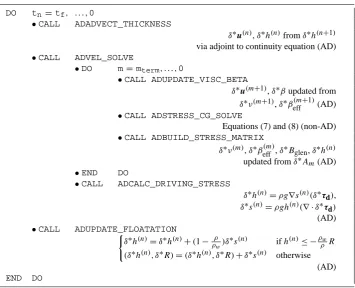
Table 3. Pseudocode version of adjoint model reverse-time-stepping algorithm corresponding to Table 1. (AD) indicates that this step is processed by the algorithmic differentiation tools.
DO tn=tf, . . . ,0
•CALL ADADVECT_THICKNESS
δ∗u(n),δ∗h(n)fromδ∗h(n+1)
via adjoint to continuity equation (AD)
•CALL ADVEL_SOLVE
•DO m=mterm, . . . ,0
•CALL ADUPDATE_VISC_BETA
δ∗u(m+1),δ∗βupdated from
δ∗ν(m+1),δ∗βeff(m+1)(AD)
•CALL ADSTRESS_CG_SOLVE
Equations (7) and (8) (non-AD)
•CALL ADBUILD_STRESS_MATRIX
δ∗ν(m),δ∗βeff(m),δ∗Bglen,δ∗h(n) updated fromδ∗Am(AD)
•END DO
•CALL ADCALC_DRIVING_STRESS
δ∗h(n)=ρg∇s(n)(δ∗τd),
δ∗s(n)=ρgh(n)(∇ ·δ∗τd)
(AD)
•CALL ADUPDATE_FLOATATION
(
δ∗h(n)=δ∗h(n)+(1− ρ
ρw)δ
∗s(n) ifh(n)≤ −ρw
ρ R
(δ∗h(n), δ∗R)=(δ∗h(n), δ∗R)+δ∗s(n) otherwise (AD)
END DO
5.1 Experiment 1: sensitivity to ice shelf stiffness
and melt rates
The first experiment does not involve optimization, but simply demonstrates the interpretive powers of the adjoint model. We consider the sensitivity of the volume of grounded ice in a marine ice stream to thermodynamic effects on its ad-jacent ice shelf. Such effects are of considerable importance, given observations of the Antarctic coastline made over the last several decades. Confined ice shelves are known to act as logjams to ice stream flow (a phenomenon referred to as ice shelf buttressing; Dupont and Alley (2005)) and there-fore exert a large control on grounded ice mass balance. The heat contained in Southern Ocean subsurface waters is able to cause melting at the underside of Antarctic ice shelves, most notably those in the Amundsen Sea embayment (Ja-cobs et al., 1996; Ja(Ja-cobs, 2006; Jenkins et al., 2010; Ja(Ja-cobs et al., 2011). Meanwhile, widespread speedup, thinning, and mass loss have been observed in these ice shelves and the ice streams that feed them (Rignot, 1998; Rignot et al., 2002; Shepherd et al., 2002, 2004).
A number of modeling studies have been carried out ex-ploring the magnitude and distribution of sub-ice shelf melt-ing that results from intrusions of warm water into an ice shelf cavity, as well as how these quantities depend on the geometry of the cavity and the strength of the
forc-ing (e.g., MacAyeal, 1984; Jenkins, 1991; Hellmer et al., 1998; Holland et al., 2008; Little et al., 2009; Heimbach and Losch, 2012). Less frequently asked is how the response of grounded ice depends on the magnitude and spatial distribu-tion of melting, though Walker et al. (2008) and Gagliardini et al. (2013) have investigated this question. To understand how large-scale changes in ocean heat content and circula-tion can affect ice sheets, both quescircula-tions are important.
Fig. 1. Background steady state of the ice stream-shelf system in Experiment 1. Coloring on
the upper surface is velocity magnitude. The thick black contour denotes the grounding line.
46
Fig. 1. Background steady state of the ice stream–shelf system in Experiment 1. Coloring on the upper surface is velocity magnitude. The thick black contour denotes the grounding line.
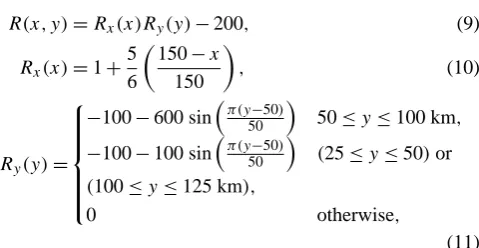
(in meters) by
R(x, y)=Rx(x)Ry(y)−200, (9)
Rx(x)=1+ 5 6
150−x
150
, (10)
Ry(y)=
−100−600 sinπ(y50−50) 50≤y≤100 km, −100−100 sinπ(y50−50) (25≤y≤50)or (100≤y≤125 km),
0 otherwise,
(11) wherex and y are in km. Sliding is governed by a linear sliding law, i.e.,
τb=β2ub. (12)
Within the channel, i.e., where 50 km≤y≤100 km,β2 is set to 30 Pa (m/a)−1. Outside of the channel it is 9 times larger. The lateral boundaries aty=0 km, 150 km are no-slip boundaries, but the resistance to ice stream flow comes from basal stress in the outer “sheet” region, not the sidewalls. The Glen’s law parameterAis set uniformly to 9.5×10⁻¹⁸ Pa−3a−1, which corresponds roughly to a temperature of −15◦C. The model is run to equilibrium, shown in Fig. 1. An ice shelf about 50 km long forms over the channel.
To examine changes in grounded ice, we consider volume above floatation (VAF), defined as volume of ice that would contribute to sea level rise if all of the ice in the domain were to melt, and the loss thereof (Dupont and Alley, 2005). Note that the floating columns of ice do not contribute to VAF. We calculate the adjoint sensitivities of VAF loss during the ten-year run to two different input fields: basal melting under the ice shelf (m˙), and the Glen’s law flow parameter A.A realistically depends on the temperature and fabric of the ice,
x (km)
y (km)
110 120 130 140
55 60 65 70 75 80 85 90 95 100
Volume loss (10
−3
km
3 (m/a) −1 )
0 0.2 0.4 0.6 0.8 1 1.2
(a)
x (km)
y
(k
m
)
20 40 60 80 100 120 140
5 10 15 20 25 30 35 40 45 50
Vo
lu
m
e
l
o
s
s
(1
0
1
5 k
m
3 Pa 3 a
)
0 1 2 3 4 5 6 7
(b)
Fig. 2. (a) Sensitivity of grounded ice volume after 10 years to sub-shelf melt rates, in km3
per (m/a) of melting. The non-colored section of the figure is within the grounded part of the domain (b) Similarly for Glen’s Law parameterA, but with units of 10−15km3Pa−3a−1. A thick
black contour denotes the grounding line. The largest values in both figures are in the ice shelf margins. Note the differingx- andy-bounds on the figures.
47
Fig. 2. (a) Sensitivity of grounded ice volume after 10 yr to sub-shelf melt rates, in 10−3 km3 per (m a−1) of melting. The non-colored section of the figure is within the grounded part of the do-main. (b) Similarly for Glen’s law parameterA, but with units of 10−15km3Pa−3a−1. A thick black contour denotes the grounding line. The largest values in both figures are in the ice shelf margins. Note the differingxandybounds on the figures.
but here we consider dependence onAdirectly. We define a scalar function
J=X
i
HAF(i)1x1y, (13)
HAF(i)=
h(i)+ρw ρ R(i)
+
, (14)
where “HAF” is height above floatation,R(i)andh(i)are bed elevation and thickness at final time in celli, and1x and1yare spacings on the (here uniform) grid.J is the cost function, or objective function, for this experiment (equal to final-time VAF), and it is the scalar function of which the gradient is found, with respect tom˙ andA, by the adjoint model.
Melt rate sensitivities are shown in Fig. 2a. The value at a location (i.e., in celli) can be interpreted as the loss in VAF after 10 yr with a constant melt rate of 1 m a−1in celli. Sen-sitivities are only nonzero in locations where ice is floating. This is due to a rule in the model that melt rates cannot be applied under grounded ice: so even though adjoint sensitiv-ities are propagated backward in time, they terminate at the point in the code where melt rates are applied. The pattern of sensitivities is interesting: they are largest not in the deep-est part of the shelf near the grounding line, where melt rates are generally highest, but rather in the margins of the shelf. This implication (which should be taken with many quali-fications, as explained below) that shifts in melt rates near relatively shallow ice shelf margins could have stronger im-pacts on grounded ice than shifts of equal magnitude near the grounding line. Also curious is the fact that sensitivities are actually negative (though very small) near the ice shelf front. This effect is in fact realized in forward runs: thinning of the ice shelf front leads to flux across the ice shelf margin (into the shelf) and drawdown of the grounded ice cliffs, lessening their contribution to VAF loss.
patterns which concentrate toward the grounding line have the greatest impact on grounded ice. However, these studies used flowline models and thus could not resolve the effects of thinning near shear margins. Therefore, this experiment high-lights the need to resolve both horizontal directions when as-sessing the impact of melting on ice shelf buttressing.
Figure 2b shows sensitivities with respect toA. (Values are large because the nominal value ofAis on the order of 10−17Pa−3a−1.) Here values are nonzero in grounded and floating ice, and are largest in the margins of the ice shelf (and negative, but small toward the ice shelf front). A is sometimes referred to as the “fluidity” of ice; i.e., the larger it is the more easily the ice flows. A positive change corre-sponds to weakening of the ice, and weakening in the mar-gins leads to the most grounded ice loss.
That the thinning (through melting) and weakening of an ice shelf can lead to grounded ice loss is well established on theoretical (Thomas, 1979) and modeling (Dupont and Alley, 2005; Goldberg et al., 2009; Little et al., 2012) bases. But less-oft discussed is which parts of the shelf are most sensi-tive to this mechanism, that is, the structural integrity of the ice shelf. The result of our idealized case, with a small, con-fined ice shelf, suggests that the margins are the weak points of the shelf. It is not clear to what extent this applies to ice shelves in general, although intuition suggests that margins play a similar role in all confined, relatively small shelves. This demonstration shows that a similar analysis can be done on any ice shelf–ice stream system (although a baseline solu-tion free of artificial model drift would be required for mean-ingful results).
The computational advantage of the adjoint in producing data sets such as those shown in Fig. 2 is considerable. Using a domain decomposition over 9 processors (with a 50×50 grid belonging to each process) took approximately 12 min-utes, or 5 seconds per time step. The adjoint run that pro-duced both data sets in Fig. 2 (and could have propro-duced ad-ditional adjoint sensitivity fields as well) took approximately 4 times longer, giving a total run time of about an hour. (The additional run time is because parts of the forward model must be run multiple times to provide state information for the reverse-time adjoint run.) If, on the other hand, one were to approximate sensitivities by perturbing single parameter values and using one-sided finite differencing, the melt rate sensitivities would take approximately 50×50×0.2 h≈25 days (since only a portion of the domain is ice shelf) and the A-sensitivities about 9 times as long.
While the efficiency of the adjoint in finding sensitivities is obvious, it should be kept in mind that the analysis is in-herently linear: a forward trajectory is needed around which to perturb. In this case the trajectory was a quiescent one, as the run began in steady state with no melting. As dis-cussed above, melting increases flux across the grounding line through loss of ice shelf buttressing; sufficiently high melt rates would lead to grounding line retreat. This, in turn, would result in increased grounding line thickness (due to the
shape of the bedrock), leading to further mass flux increase (Schoof, 2007). The latter effect is nonlinear, however, and is not detected by our adjoint results. When calculating adjoint sensitivities, the results should not be taken at face value, but rather serve as a starting point for further investigation. It is worth noting that Goldberg et al. (2012b), using a cou-pled ice–ocean model that allowed grounding line migration, found that thinning of an ice shelf at the margin due to melt-ing was a key factor in unstable retreat of grounded ice – giv-ing credence to the high sensitivities of VAF loss to values in the ice shelf margin.
5.2 Experiment 2: inversion of basal sliding coefficients
from surface velocities
In our first inversion experiment we infer basal sliding coeffi-cients from surface velocities, considering only the momen-tum balance of the model (i.e., no time dependence). This is an identical-twin experiment, in that the surface velocities come from model output with prescribed parameter values (or “true” values), and the inverted parameters are then com-pared with the truth. The forward model is one-dimensional (only one horizontal direction is considered, and the SSA bal-ance is implemented) with periodic boundary conditions, and surface slope and thickness are constant.
Many authors have carried out similar inversions over the past two decades, both with synthetic observations and real ones (e.g., MacAyeal, 1992, 1993; Vieli and Payne, 2003; Khazendar et al., 2007; Sergienko et al., 2008; Morlighem et al., 2010; Joughin et al., 2009). The purpose of this ex-periment is not to introduce a new type of glaciological in-version, or to improve upon an existing one, but rather to enable direct comparison with existing methods. As one of the simplest glaciological inverse problems, our adjoint opti-mization framework must, at a minimum, perform as well as other inversion methods.
The experiment is based on Experiment B from the ISMIP-HOM intercomparison (Pattyn et al., 2008) withL= 40 km, and 1 km resolution. The intercomparison specifies a constant thickness of 1000 m, a constant surface slope of 0.1◦, and a linear sliding law with a mode-one sinusoidally varying sliding coefficient, or lubrication,β2(Fig. 3a). This profile ofβ2represents our true parameter values. The Glen’s law parameterAis uniformly set to 10−16 Pa−3m a−1. We define asu∗
1 thex velocities from the model with these pa-rameters.
For the inverse problem to determineβ2, we define a cost function on the model output:
J=1 2
N
X
i
(u∗1(i)−u(i))2
σi2 , (15)
0 5 10 15 20 25 30 35 40 0
1000 2000
x (km)
β
2 (Pa (m/a) −1)
0 5 10 15 20 25 30 35 40
0 30 60
vel (m/a)
∂ s/∂ x = −.0017
∂ s/∂ x = −.0087 (× 0.1)
(a)
0 20 40 60 80 100
10−2
100
102
104
106
iter #
J
Adjoint model Approx. adjoint
(b)
0 20 40 60 80 100
100
102
104
106
iter #
J
Adjoint model Approx. adjoint
(c)
0 5 10 15 20 25 30 35 40
0 200 400 600 800 1000
x (km)
δβ
(1st iteration)
0 5 10 15 20 25 30 35 40
−0.4 0 0.4
x 105
δβ
(2nd iteration)
Adjoint model Approx. adjoint
(d)
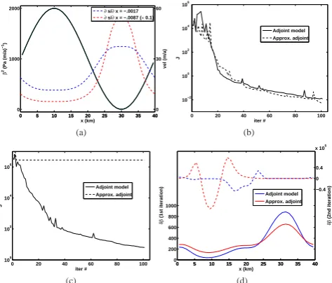
Fig. 3. (a) Data for inverse problem. ”True” basal sliding coefficientβ2
true(left axis) and
corre-sponding velocity profiles (right axis) for low and high surface slopes. (b) Cost functionJversus number of model evaluations for full and approximate adjoint, low surface slope. (c) Same for high surface slope. (d) Gradient found by full and approximate adjoint in first iteration (solid) and second iteration (dashed), high surface slope.
48
Fig. 3. (a) Data for inverse problem. “True” basal sliding coefficient βtrue2 (left axis) and corresponding velocity profiles (right axis) for low and high surface slopes. (b) Cost functionJ versus number of model evaluations for full and approximate adjoint, low surface slope. (c) Same for high surface slope. (d) Gradient found by full and approximate adjoint in first iteration (solid) and second iteration (dashed), high surface slope.
the current guess forβ through the stress balance. (In this inversion, we attempt to recoverβ, notβ2, which is the eas-iest way to impose the constraint that sliding coefficients are nonnegative.) The numbersσiare scaling factors for the cost function. Generally these scaling factors represent a priori knowledge or first guesses regarding observations or param-eters; for instance,σi might be the uncertainty in the velocity observation. In practice, this prevents poorly constrained ob-servations from leading to overspecification. In this example, the scaling factors are set uniformly to 1: this presents no loss of generality, as long as values ofJ are compared to the ini-tial value.
For a givenβ, the adjoint finds sensitivities ofJ with re-spect toβ. The cost function is then minimized using the op-timization algorithm described in Sect. 4. Notice that no reg-ularization terms have been added to the cost function to en-sure a priori properties of the lubrication field, e.g., smooth-ness and boundedsmooth-ness, although we include such terms in later experiments.
Figure 3b shows howJ evolves, eventually reaching cost reduction, defined asJJ
0
, on the order of 10−6.J0 is the value ofJ using the initial guess for β2(described below). For comparison, an inversion is also carried out where the “approximate” adjoint of MacAyeal (1993) is used, rather than the adjoint sensitivities from the AD-generated adjoint (the “full” adjoint). The approach is termed approximate be-cause the dependence of viscosity on strain rates is ignored.
In both cases, the same optimization algorithm is used, so calculated adjoint sensitivities are the only difference be-tween the two inversions.
The invertedβ2 is not shown, but it is very close to the true profile. The same is true of the experiment with higher surface slope, described below. This is because of the lack of high-frequency variability in the initial guess. If the initial guess had a broad spectrum with power at high frequencies, such as a Gaussian shape (not shown), the inversion would still decreaseJas in Fig. 3b, and the invertedβ2would have the same broad pattern as the true profile, but there would be high-frequency variability as well. This is because the veloci-ties in the model are insensitive to high-frequency variability inβ2; they are muted by longitudinal stresses.
Both optimizations begin with the same initial guess for β2, a half-mode sinusoid of the same amplitude. A uniform βwould be the simplest guess, but with a constant thickness and surface slope there is zero strain rate, and this leads to very high values for viscosity. The performance of the in-verse model then depends on the viscosity regularization pa-rameter. With the hybrid balance, this is not an issue; but in this experiment the SSA balance is used so that different in-version approaches can be compared.
The full and approximate adjoints perform equally well in the experiment with a surface slope of 0.1◦, with the full adjoint actually leading to greater values ofJ early on. However, when surface slope is increased to 0.5◦ (as in the ISMIP-HOM experiments with flow over a wavy bed), their performances differ. Now the target surface velocitiesu∗5(i) are an order of magnitude larger (Fig. 3a), and it is important to maintain the nonlinear dependence of viscosity on strain rates in the adjoint, as evidenced by the poor performance of the approximate adjoint (Fig. 3c). This can also be seen by examining the adjoint sensitivities from the two models. Af-ter the first iAf-teration of the inversion (Fig. 3d) the sensitivity profiles are similar, yielding similar search directions in the optimization algorithm. On the next iteration, however, the profiles look very different, and upon being provided with the approximate adjoint sensitivities, the optimization algo-rithm is unable to lower the cost function.
This is not to say that the AD-generated adjoint model is in all cases an improvement over the approximate adjoint in this type of inversion. The optimization algorithm has a number of associated parameters; it is possible that, for the experi-ment considered, different parameters might yield better per-formance with the approximate adjoint, or worse with the full adjoint. It is clear, nevertheless, that instances exist where the full adjoint is advantageous.
5.3 Experiment 3: estimation of past conditions
x (km)
elev (m)
0 0.5 1 1.5 2 2.5 3 3.5 4
x 104
0 200 400 600 800 1000 1200 1400 1600 1800 2000 (a) x (km) y (km)
5 10 15 20 25 30 35
5 10 15 20 25 30 35 β
2 (Pa (m/a) −1) 300 400 500 600 700 800 900 (b) 0 10 20 30 40 0 20 40 990 995 1000 1005 1010 x (km) y (km) h (m) (c) x (km) y (km)
5 10 15 20 25 30 35
5 10 15 20 25 30 35 speed (m/a) 98 100 102 104 106 108 110 112 114 116 118 120 (d)
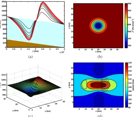
Fig. 4. (a) ”True” profile of glacier at timet= 0and transient surface profiles spaced one year, exaggerated by a factor of 100. The last 5 profiles (in red) correspond to data used to constrain
β2andh(t= 0). (b) ”True”β2. (c) Thickness at final time (t= 10a). (d) Surface speed at final
time. Region where flow is strongly divergent (convergent) is indicated by solid (dotted) black contours.
49
Fig. 4. (a) “True” profile of glacier at timet=0 and transient sur-face profiles spaced one year, exaggerated by a factor of 100. The last 5 profiles (in red) correspond to data used to constrainβ2and
h(t=0). (b) “True”β2. (c) Thickness at final time (t=10 a). (d) Surface speed at final time. Region where flow is strongly divergent (convergent) is indicated by solid (dotted) black contours.
(2011). However, the assimilation in this study consisted of a series of “snapshot” inversions of surface velocities; no dy-namic consistency between the states at different times was enforced. We re-emphasize that the propagation of sensitiv-ity/misfit information back in time by the adjoint model im-plies that the inversion takes advantage of available observa-tions not only forward in time (as do filter or sequential as-similation methods) but also backward in time (smoother or variational methods), mediated through the model dynamics. We consider a mountain glacier undergoing adjustment in response to a perturbation in basal conditions. We assume we have knowledge of surface velocities at the end of this adjustment (the “present”) and of thickness and surface el-evations at certain discrete times during the adjustment, but not of the initial thickness, nor of the basal conditions dur-ing this adjustment. Perfect knowledge of bed elevation is also assumed (this is not, in general, the case, and in the next experiment we deal with bed topography uncertainty). We ask whether we can recover this initial thickness and basal traction with adjoint-based optimization. Reconstructions of past glacier configuration, coupled with inversions of basal properties, could be very useful in certain glaciological set-tings. For instance, if an ice stream is known to be out of balance due to relatively recent changes in its basal environ-ment, such an inversion could give us thickness of the stream prior to its observational history or, conversely, could pin-point the time of onset of the changes.
The forward model is again a periodic domain with a con-stant bed slope of−0.5◦ in the x direction. Both
horizon-0 50 100 150 200 250 300
10−2 100 102 104 iter # J (a) 0 10 20 30 40 0 20 40 990 995 1000 1005 1010 x (km) y (km) h (m) (b) 0 10 20 30 40 0 20 40 990 995 1000 1005 1010 x (km) y (km) h (m) (c) 0 10 20 30 40 0 20 40 990 995 1000 1005 1010 x (km) y (km) h (m) (d)
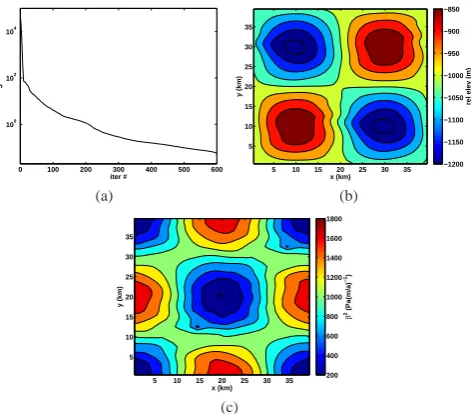
Fig. 5. (a) Value of cost function versus iteration. (b) Final inverted initial thickness (h(t= 0)). ”True” field is uniformly 1000 m. Compare with Fig. 4(c), which is used as the initial guess. Maximum misfit is reduced from 9 m to 1.8 m;r.m.s.misfit is reduced from 2.6 m to 0.25 m. (c) Inverted initial thickness when velocity is ”frozen” in its observed state (Fig. 4(d)). (d) Inverted initial thickness when only the observed thickness att= 10 years is used to constrain the problem.
50
Fig. 5. (a) Value of cost function versus iteration. (b) Final inverted initial thickness (h(t=0)). “True” field is uniformly 1000 m. Com-pare with Fig. 4c, which is used as the initial guess. Maximum mis-fit is reduced from 9 to 1.8 m; rms mismis-fit is reduced from 2.6 to 0.25 m. (c) Inverted initial thickness when velocity is "frozen" in its observed state (Fig. 4d). (d) Inverted initial thickness when only the observed thickness att=10 yr is used to constrain the problem.
tal dimensions are resolved, and the domain isy periodic as well, with zero bed slope in they direction. The domain is 40×40 km with 1 km resolution. The initial thickness is uni-form with a value ofH0=1000 m. The Glen’s law parameter Ais as in the previous experiment. A hybrid stress balance is used. The sliding law is again linear, with sliding coefficient β2. The trueβ2is defined as
β2=1000−750 exp
− r 5 2 , (16)
with units of Pa m a−1, where r is distance from the center of the domain in km. The model is integrated forward with 30-day time steps for 10 yr, at the end of which the model is close to a new equilibrium. Figure 4a shows the initial surface and thickness, as well as annual surface elevations during the adjustment (magnified a hundred-fold), along the center liney=20 km.
For data in our identical-twin inversion to recoverβ2and the initial thickness, we take annual surface elevation over the last 5 yr (the red curves in Fig. 4a) and surface velocity averaged over the last year (Fig. 4d). These are referred to below as the “target data”. We define a cost function
J= N X
i
1 N σ2
u
|us∗(i)−us(i)|2+
1 N σ2
s
10
X
n=6
s(n),∗(i)−s(n)(i)2 !
since the observations are synthetic there is no rationale to use spatially varying uncertainties. The relative values ofσu andσs affect the results of the inversion, however. We use 1 m/a forσuand 2 cm for σs. Thus whenJ∼O(1) then the model misfit is on the order of observational uncertainties on average. This value is motivated by the spread of surface ele-vations over the 5 yr sampling period; field measurements of surface elevation generally have O(∼1 m) errors, at least in relatively flat regions (Griggs and Bamber, 2008). GPS mea-surements are capable of much higher accuracy than remote sensing, provided the presence of a nearby exposed promon-tory, or ice for which the surface elevation is changing on much slower timescales (N. Gourmelen, personal commu-nication, 2013), but we concede that GPS observations are unlikely to be collected with such high spatial resolution.
For initial guesses, a uniform value of βguess2 ≡ 400 Pa m a−1is used forβ2; as forh(0), the observed thick-ness att=10 yr is used. That is,
h(0)guess=R+s(10),∗ (18)
whereR is the bedrock, the rationale being that, in this arti-ficial experiment, the glacier is in this configuration (or close to it) during the period of observation.
Figure 5a shows the cost function trajectory. About 60 to 80 gradient evaluations are required forJ to be O(1), but the inversion is carried farther than that. Figure 5b shows the final estimate ofh(0). Remnants of the initial guess can be seen, but the associated misfit (when compared with the true h(0)) has a maximum amplitude of about 1.8 m, whereas that of the initial guess has a maximum of 9 m. In terms of root mean square error,
errrms=
(h(0)−1000)2 1/2
, (19)
this value is reduced from 2.6 m for the initial guess to 0.25 m. The estimatedβ2 is not shown; it differs from the trueβ2by at most 2 %.
To appreciate the complexity of this inverse problem, one should contrast with that of reconstructing the history of an advected field in a flow that is fixed, or independent of the field. Such problems have been dealt with frequently in generic flow fields. Our problem is more complex, in that the velocities depend nonlinearly and nonlocally on the advected quantity (thickness). To illustrate this, another experiment is carried out, in which depth-averaged velocity is fixed to the target surface velocity, independent of time. The cost func-tion consists only of the second term in Eq. (17), and the only control field is initial thickness, with initial guess the same as before. The forward model is essentially just the mass bal-ance equation. The estimatedh(0)is shown in Fig. 5c. In this experiment the cost function only decreases by a factor of 20 (as opposed to the O(106) decrease shown in Fig. 5a). More interesting is that the final estimate ofh(0)is actually worse than the initial guess. This is because the divergence pattern
in the target velocity field (Fig. 4d) differs from that through-out much of the “truth” simulation.
It is also interesting to consider how the time dependence of the constraints affects the inversion. The forward model is close to steady state by the end of the 10 yr integration, and the observed surface fieldss(n),∗ differ on the order of centimeters. Since they are so close, one might guess that constraining the surface at years 6 through 9 of the simula-tion adds little informasimula-tion beyond that contained in the sur-face elevation at year 10. However, this is not the case. We carry out another inversion in which the cost function given by Eq. (17) is modified so that the summation overn only contains one term,n=10. That is, only the final surface ele-vation is constrained. In this experiment, the stress and mass balances are again used, rather than solely the mass balance. Figure 5d shows the result of this inversion. In this case the estimated initial thickness is much closer to the initial guess than the trueh(0). Valuable information about the thickness trajectory is contained in the intermediate surface observa-tions, even though the temporal variability is small. This par-ticular result hinges on a level of measurement accuracy that is not generally attained; still, it demonstrates the importance of time-dependent information in estimating past ice sheet behavior and other unknown parameters.
To our knowledge, a similar inversion experiment has not been carried out with a higher-order model; although numer-ical inversions for historic data, including prior ice thick-nesses, have been carried out using a model that makes the shallow ice approximation (e.g, Waddington et al., 2007). For this reason, Experiment 3 is intended as a preliminary in-vestigation in inferring unknown parameters based on time-dependent data, in which different types of data (surface el-evation and velocities) are not co-temporal. There are many other questions that can be asked of such inversions: for in-stance, how is the inversion affected if data is not spatially complete, and if the “holes” in data at different times are not coincident? Does the quality of the estimation decay with the hindcast horizon? The choice of duration of our experiment was based on the adjustment time of the forward model, but it is unclear at which point the signal of observations gets lost in the noise of the model. Also, we did not allow for time-dependent lubrication, as in Jay-Allemand et al. (2011); how does this affect the ease of solution?
5.4 Experiment 4: simultaneous inversion of basal topography and sliding coefficients
Two prevalent challenges in modeling dynamic behavior of real glaciers and ice sheets are those of basal topography and of model initialization. Basal topography is often collected by sparse flight lines of airborne ice-penetrating radar, lead-ing to very low-resolution representations of ice thickness much lower than that required by models used to study highly dynamic features such as ice streams. Recent published er-rors of gridded Antarctic ice thickness uncertainty are tens of meters or more (e.g., Fretwell et al., 2013). Given the sen-sitivity of models to representations of bed topography (Du-rand et al., 2011; Seroussi et al., 2011), this introduces large uncertainties into model response.
Model initialization is important for studies that aim to as-sess the time-dependent response of ice sheets and glaciers in their current configurations to external forcing. In these studies it is important to start from a quasi-balanced state, in which there is no unrealistic model adjustment or drift that will contaminate the results. Long-timescale spinups can be computationally expensive, and due to parameter uncertainty there is no guarantee that the steady state produced is close to the observed state.
A number of studies have made use of the adjoint method introduced by MacAyeal (1993) to estimate these parameters. However, these inversions are problematic in that the various data sets used are gathered using different methods and res-olutions at different times. Very often the sres-olutions can lead to large anomalous mass balances when used to initialize a time-dependent model. Contributing greatly to the error in-herent in the inverted solutions are the uncertainties in basal topography (Morlighem et al., 2011).
Two related issues emerge: uncertainties in ice thickness and basal topography, and their impact on the usefulness of assimilated products in model initialization. To deal with the latter, some studies run spinups (albeit shorter ones due to improved parameter guesses) or add “flux corrections” in the term of surface or basal mass balances (e.g., Joughin et al., 2009; Larour et al., 2012a). Such approaches are not ideal, because the model response may be influenced by the ad-justed configuration or artificial mass balance. Morlighem et al. (2011) carries out an adjoint-based method that is con-strained by the continuity equation with observed velocities, thus guaranteeing a stable mass balance. Basal lubrication and ice stiffness can then be estimated using other methods. However, the method does not consider the stress and mass balance equations together, and thus it does not truly provide a balanced state. In particular, the resulting model velocities may agree well with observed velocities in theL2-norm, but this does not guarantee that the divergence patterns will be identical.
With a time-dependent ice model adjoint it is possible to constrain both the continuity equation and the momentum equations in simultaneous inversions for basal lubrication
and topography. In this section we explore the potential of using this approach both to minimize drift in model initializa-tions and to provide improved estimates of basal topography. We note that methods for such inversions have been previ-ously developed (Thorsteinsson et al., 2003; Gudmundsson and Raymond, 2008). However, these methods assume New-tonian rheology and rely on linear transfer functions of small perturbations, so it is not clear that their results carry over to large deviations and nonlinear rheologies.
We also point out that, in the general case, the retrieval of basal lubrication and topography is ill-posed. Consider a slid-ing glacier of infinite extent, with constant thickness, surface slope, and basal lubrication. With negligible horizontal ve-locity divergence, the glacier would be in steady state. There are an infinity of lubrication/bed elevation parameter pairs that would give the same surface velocity with the given sur-face elevation. This is an extreme case, but we will keep this potential limitation in mind. On a related note, the degree to which existing studies of inversions for basal lubrication have compensated for errors in bed topography has remained largely unquantified.
5.4.1 Uncertainties in bed elevation
We perform an identical-twin experiment, in which the sur-face elevation and velocity are known for an idealized glacier in steady state. This steady state is found by time-integrating the model in a doubly periodic, 40×40 km domain. A linear sliding law is used, with sliding coefficientβ2. Bed topog-raphy and lubrication are given very simple analytical pre-scriptions, with single-wavelength variation in bothx andy directions:
R(x, y)=R0(x)+200 sin
2πy
40
sin
2π x
40
, (20)
β2(x, y)=1000−800 cos
2πy
40
cos
2π x
40
, (21)
given in units of m and Pa (m/a)−1, respectively, wherexand y are in km andR0(x)gives a constant downward slope of 0.5◦ in thex direction. The Glen’s law coefficient is as in
x (km)
y (km)
5 10 15 20 25 30 35
5 10 15 20 25 30 35
rel elev (m)
−1200 −1150 −1100 −1050 −1000 −950 −900 −850 (a) x (km) y (km)
5 10 15 20 25 30 35
5 10 15 20 25 30 35 β
2 (Pa(m/a) −1) 200 400 600 800 1000 1200 1400 1600 1800 (b) x (km) y (km)
5 10 15 20 25 30 35
5 10 15 20 25 30 35
rel elev (m)
−20 −15 −10 −5 0 5 10 15 20 (c) x (km) y (km)
5 10 15 20 25 30 35
5 10 15 20 25 30 35 speed (m/a) 85 90 95 100 105 110 115 120 125 130 135 (d)
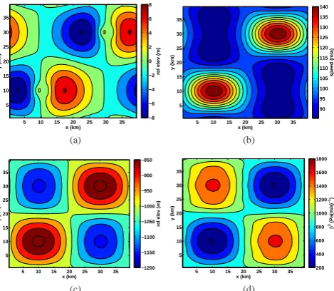
Fig. 6. (a) True basal topographyRin Experiment 4, with constant trend inx-direction removed. (b) Trueβ2in Experiment 4. (c) Steady-state surface elevation, linear trend removed. (d) Ice
surface speed corresponding to steady state.
51
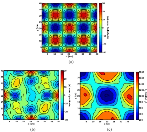
Fig. 6. (a) True basal topographyR in Experiment 4, with con-stant trend inx-direction removed. (b) Trueβ2in Experiment 4. (c) Steady-state surface elevation, linear trend removed. (d) Ice surface speed corresponding to steady state.
We set up our identical-twin experiment by assuming per-fect knowledge of surface elevation and surface velocity, and little or no information about basal topography and basal lu-brication, aside from their general scales. We define a cost function
J = 1
N σ2
u
PN
i |us∗(i)−us(i)|2+N 1tγd2
PN
i
h(1)(i)−h(0)(i)2+γo
Nk∇h (0)k2
+γbPNi exp
β(i)2 β2 max , (22)
where the summation is over all cellsi. The forward model runs for a single time step, andus andh(1) are the model surface velocity and thickness after that time step.us∗is the observed surface velocity shown in Fig. 6d. The first term in Eq. (22) penalizes misfit with observed velocities.σu is as in Sect. 5.3. The second term penalizes model drift, i.e., the amount by which thickness changes over the single time step. If we were constraining the rate of thickness change to be close to a nonzero observed rate, the term would be different, but here we are constraining the model to be close to steady state.γd is chosen so that the term is order unity when thickness rate of change is on the order of 10−4.
The third and fourth terms in (Eq. 22) pertain to the “model” norm, rather than the misfit norm (Waddington et al., 2007), meaning they deal with a priori knowledge of the unknown parameters. The third term is a simple Tikhonov smoothing term that penalizes large oscillation in thickness (and bed topography; see below). The norm|·|is that induced by summing the square of the centered finite difference ap-proximation to the gradient over all cells.γois chosen so that the term only makes a contribution if thickness gradients are
0 100 200 300 400 500 600
100 102 104 iter # J (a) x (km) y (km)
5 10 15 20 25 30 35
5 10 15 20 25 30 35
rel elev (m)
−1200 −1150 −1100 −1050 −1000 −950 −900 −850 (b) x (km) y (km)
5 10 15 20 25 30 35
5 10 15 20 25 30 35 β
2 (Pa(m/a)
−1 ) 200 400 600 800 1000 1200 1400 1600 1800 (c)
Fig. 7. Inversion for basal topography and lubrication with uniform initial guesses (basal
eleva-tionR≡-1000 m,β2≡400 Pa(m/a)−1) . (a) Cost function versus forward and adjoint iteration
number. (b) Inverted basal topography; compare with Fig. 6(a).rmserror is 5.9 m, compared
with an initial value of 100 m. (c) Invertedβ2.
52
Fig. 7. Inversion for basal topography and lubrication with uniform initial guesses (basal elevationR≡-1000 m,β2≡400 Pa m a−1). (a) Cost function versus forward and adjoint iteration number. (b) Inverted basal topography; compare with Fig. 6a. rms error is 5.9 m, compared with an initial value of 100 m. (c) Invertedβ2.
larger than∼0.1 on average. The fourth term penalizes basal lubrication if it becomes too large during the minimization. It was found that without this term, the minimization algorithm can sometimes favor extremely large values ofβ2in favor of making adjustments to initial thickness, and this term helps to prevent that. For the experiment shown here this term was found not to be necessary.
The basal lubricationβ and the bed elevation R are the control variables in the minimization of Eq. (22). The surface elevation,s, is constrained to be that of the computed steady state, sss (the same as that shown in Fig. 6c). Rather than penalizing the misfit of s in the cost function, the surface elevation is controlled exactly through the initial guess for ice thickness. That is, the initial guess for thickness,h(0)guess, and topography,Rguess, are defined such that
h(0)guess+Rguess=sss. (23)
When the guess for R is updated by a function δR, the topographyh(0)is updated by−δR.
The initial guesses for basal lubrication and topography are
βguess2 (x, y)≡400 Pa(m/a)−1, (24)
Rguess(x, y)=R0(x). (25)