https://doi.org/10.5194/cp-13-1539-2017 © Author(s) 2017. This work is distributed under the Creative Commons Attribution 3.0 License.
Emulation of long-term changes in global climate:
application to the late Pliocene and future
Natalie S. Lord1,2, Michel Crucifix3,4, Dan J. Lunt1,2, Mike C. Thorne5, Nabila Bounceur3,6, Harry Dowsett7, Charlotte L. O’Brien8, and Andy Ridgwell1,2,9
1School of Geographical Sciences, University of Bristol, Bristol, BS8 1SS, UK 2Cabot Institute, University of Bristol, Bristol, BS8 1UJ, UK
3Université catholique de Louvain, Georges Lemaître Centre for Earth and Climate Research, Earth and Life Institute,
1348 Louvain-la-Neuve, Belgium
4Belgian National Fund for Scientific Research, Brussels, Belgium
5Mike Thorne and Associates Limited, Quarry Cottage, Hamsterley, Bishop Auckland, Co. Durham, DL13 3NJ, UK 6Department of Applied Mathematics and Computational Science, King Abdullah University of Science and Technology,
Thuwal. 23955-6900, Kingdom of Saudi Arabia
7Eastern Geology and Paleoclimate Science Center, US Geological Survey, Reston, VA 20192, USA 8Department of Geology and Geophysics, Yale University, New Haven, CT 06511, USA
9Department of Earth Sciences, University of California, Riverside, CA 92521, USA
Correspondence to:Natalie S. Lord ([email protected])
Received: 4 April 2017 – Discussion started: 26 April 2017 Accepted: 6 October 2017 – Published: 16 November 2017
Abstract.Multi-millennial transient simulations of climate changes have a range of important applications, such as for investigating key geologic events and transitions for which high-resolution palaeoenvironmental proxy data are avail-able, or for projecting the long-term impacts of future climate evolution on the performance of geological repositories for the disposal of radioactive wastes. However, due to the high computational requirements of current fully coupled general circulation models (GCMs), long-term simulations can gen-erally only be performed with less complex models and/or at lower spatial resolution. In this study, we present novel long-term “continuous” projections of climate evolution based on the output from GCMs, via the use of a statistical emulator. The emulator is calibrated using ensembles of GCM simu-lations, which have varying orbital configurations and atmo-spheric CO2concentrations and enables a variety of
investi-gations of long-term climate change to be conducted, which would not be possible with other modelling techniques on the same temporal and spatial scales. To illustrate the potential applications, we apply the emulator to the late Pliocene (by modelling surface air temperature – SAT), comparing its re-sults with palaeo-proxy data for a number of global sites, and
to the next 200 kyr (thousand years) (by modelling SAT and precipitation). A range of CO2 scenarios are prescribed for
each period. During the late Pliocene, we find that emulated SAT varies on an approximately precessional timescale, with evidence of increased obliquity response at times. A compar-ison of atmospheric CO2 concentration for this period,
es-timated using the proxy sea surface temperature (SST) data from different sites and emulator results, finds that relatively similar CO2 concentrations are estimated based on sites at
emula-tor to capture deviations from a quasi-stationary response to the forcing, such as transient adjustments of the deep-ocean temperature and circulation, in addition to its limited range of fixed ice sheet configurations and its requirement for pre-scribed atmospheric CO2concentrations.
1 Introduction
Palaeoclimate natural archives reveal how the Earth’s past climate has fluctuated between warmer and cooler inter-vals. Glacial periods, such as the Last Glacial Maximum (e.g. Lambeck et al., 2000; Yokoyama et al., 2000), ex-hibit relatively lower temperatures associated with extensive ice sheets at high northern latitudes (Herbert et al., 2010; Jouzel et al., 2007; Lisiecki and Raymo, 2005), whilst in-terglacials are characterized by much milder temperatures in global mean. Even warmer and sometimes transient (“hyper-thermal”) intervals, such as occurred during the Palaeocene– Eocene Thermal Maximum (e.g. Kennett and Stott, 1991), are characterized by even higher global mean temperatures. Assuming that on glacial–interglacial timescales and across transient warmings and climatic transitions tectonic effects can be neglected, the timing and rate of climatic change is at least partly controlled by the three main orbital param-eters – precession, obliquity and eccentricity – which have cycle durations of approximately 23, 41, and both 96 and ∼400 kyr (thousand years), respectively (Berger, 1978; Hays et al., 1976; Kawamura et al., 2007; Lisiecki and Raymo, 2007; Milankovitch, 1941). Further key drivers of past cli-mate dynamics include changes in atmospheric CO2
con-centration and in respect of the glacial–interglacial cycles, changes in the extent and thickness of ice sheets.
In order to investigate the dynamics, impacts and feed-backs associated with the response of the climate system to orbital forcing and CO2, long-term (>103yr – years)
projec-tions of changing climate are required. Transient simulaprojec-tions such as these are useful for investigating key past episodes of extended duration for which detailed palaeoenvironmental proxy data are available, such as through the Quaternary and Pliocene, allowing data–model comparisons. Simulations of long-term future climate change also have a number of ap-plications, such as in assessments of the safety of geolog-ical disposal of radioactive wastes. Due to the long half-lives of potentially harmful radionuclides in these wastes, geological disposal facilities must remain functional for up to 100 kyr in the case of low- and intermediate-level wastes (e.g. Low Level Waste Repository, UK; LLWR, 2011), and up to 1 Myr in the case of high-level wastes and spent nuclear fuel (e.g. proposed KBS-3 facility, Sweden; SKB, 2011). Projections of possible long-term future climate evolution are therefore required in order for the impact of potential climatic changes on the performance and safety of a reposi-tory to be assessed (NDA, 2010; Texier et al., 2003). Indeed, while the glacial–interglacial cycles are expected to continue
into the future, the timing of onset of the next glacial episode is currently uncertain and will be fundamentally impacted by the increased radiative forcing from anthropogenic CO2
emissions (Archer and Ganopolski, 2005; Ganopolski et al., 2016; Loutre and Berger, 2000b).
Making spatially resolved past or future projections of changes in surface climate generally involves the use of fully coupled general circulation models (GCMs). However, a consequence of their high spatial and temporal resolution and structural complexity (and attendant computational re-sources) is that it is not usually practical to run them for simulations of more than a few millennia, and invariably, rather less than a single precessional cycle. Even when run for several thousand years, only a limited number of runs can be performed. Previously, therefore, lower-complexity models such as Earth system Models of Intermediate Com-plexity (EMICs) have been used to simulate long-term tran-sient past (e.g. Loutre and Berger, 2000a; Stap et al., 2014) and future (e.g. Archer and Ganopolski, 2005; Eby et al., 2009; Ganopolski et al., 2016; Lenton et al., 2006; Loutre and Berger, 2000b) climate development. Where GCMs have been employed, generally only a relatively small number of snapshot simulations of particular climate states or time slices of interest have been modelled (e.g. Braconnot et al., 2007; Haywood et al., 2013; Marzocchi et al., 2015; Masson-Delmotte et al., 2011; Prescott et al., 2014).
In this study, we present long-term continuous projections of climate evolution based on the output from a GCM, via the use of a statistical emulator. Emulators have been utilised in previous studies for a range of applications, including sen-sitivity analyses of climate to orbital, atmospheric CO2 and
ice sheet configurations (Araya-Melo et al., 2015; Bounceur et al., 2015) and model parameterisations (Holden et al., 2010). However, to the best of our knowledge, this is the first time that an emulator has been trained on data from a GCM and then used to simulate long-term future transient climate change. It should be noted that, whilst other research communities may use different terms, we refer to the groups of climate model experiments as “ensembles”, and we refer directly to the GCM when discussing calibration of the emu-lator, rather than using the term “simulator” as has been used in a number of previous studies.
We calibrated an emulator using surface air temperature (SAT) data produced using the HadCM3 GCM (Gordon et al., 2000). Two ensembles of simulations were run, with varying orbital configurations and atmospheric CO2
asso-ciated with this approach are discussed in Sect. 7. The ensem-bles thus cover a range of possible future conditions, includ-ing the high atmospheric CO2 concentrations expected in
the near-term due to anthropogenic CO2emissions, and the
gradual reduction of this CO2 perturbation over timescales
of hundreds of thousands of years by the long-term carbon cycle (Lord et al., 2015, 2016).
We go on to illustrate a number of different ways in which the emulator can be applied to investigate long-term climate evolution over hundreds of thousands to millions of years. Firstly, the emulator is used to simulate SAT changes for the late Pliocene for the period 3300–2800 kyr BP (before present) for a range of CO2concentrations. This interval
oc-curs in the middle part of the Piacenzian age, and was pre-viously referred to as the “mid-Pliocene” (e.g. Dowsett and Robinson, 2009). During this time, global temperatures were warmer than pre-industrial (e.g. Dowsett et al., 2011; Hay-wood and Valdes, 2004; Lunt et al., 2010), before the transi-tion to the intensified glacial–interglacial cycles that are asso-ciated with Quaternary climate (Lisiecki and Raymo, 2007). We then apply the emulator to future climate, simulating tem-perature and precipitation data for the next 200 kyr AP (after present) for a range of anthropogenic CO2emissions
scenar-ios. Regional changes in climate at a number of European sites (grid boxes) are presented, selected either because they have been identified as adopted or proposed locations for the geological disposal of solid radioactive wastes, as in the cases of Forsmark, Sweden, and El Cabril, Spain, or simply as ref-erence locations where a suitable site has not yet been iden-tified, as in the cases of Switzerland and the UK.
The paper is structured such that the theoretical basis of the emulator is described in Sect. 2, the GCM model description and simulations are presented in Sect. 3 and an account of how the emulator is trained and evaluated is given in Sect. 4. Section 5 presents illustrative examples of a number of po-tential applications of the emulator for the late Pliocene. Fur-ther examples of the application of the emulator to the next 200 kyr are described in Sect. 6. Section 7 includes a de-scription and discussion of uncertainties associated with the methodology and tools, and the conclusions of this study are presented in Sect. 8.
2 Theoretical basis of the emulator
The emulator is a statistical representation of a more complex model, in this case a GCM. It works on the principle that a relatively small number of experiments, which fill the entire multidimensional input space (in our case, four dimensions consisting of three orbital dimensions and a CO2dimension),
albeit rather sparsely, are carried out using the GCM. The statistical model is calibrated on these experiments, with the aim of being able to interpolate the GCM results such that it can provide a prediction of the output that the GCM would produce if it were run using any particular input
configura-tion (i.e. any set of orbital and CO2conditions). If successful
(as can be tested by comparing emulator results with addi-tional GCM results not included in the calibration), no fur-ther experiments are required using the GCM; the emulator can then be used to produce results for any set of conditions or sequence of sets of conditions within the range of condi-tions on which it has been calibrated. It should not, of course, be used to extrapolate to conditions outside that range.
In this study, we use a principal component analysis (PCA) Gaussian process (GP) emulator based on Sacks et al. (1989), with the subsequent Bayesian treatment of Kennedy and O’Hagan (2000) and Oakley and O’Hagan (2002), and a PCA approach associated with Wilkinson (2010). All code for the GP package is available online at https://github.com/ mcrucifix/GP. This principal component (PC) emulator is based on climate data for the entire global grid, as opposed to calibrating separate emulators based on data for individual grid boxes. This approach is taken because, for past climate, the global response overall is of interest, rather than just the response at specific locations individually. It also means that the results are consistent across all locations. For future climate, and in particular for application to nuclear waste, recommendations and results should be consistent across all sites, which would be especially relevant to a large country such as the US. Alternatively, for some countries and loca-tions, it may be more appropriate to emulate specific grid boxes. The theoretical basis for the emulator and its calibra-tion is as follows.
Let D represent the design matrix of input data with n rows, where n is the total number of experiments per-formed with the GCM, here 60 (sum of the two ensembles). The number of columns,p, is defined by the number of di-mensions in input parameter space. In this case,p=4 rep-resenting the three orbital parameters and atmospheric CO2
concentration. A more detailed explanation of the orbital in-put parameters is included in Sect. 3; however, briefly, they are longitude of perihelion ($), obliquity (ε) and eccentric-ity (e), with longitude of perihelion and eccentricity being combined under the formesin$ andecos$. For a set of i=1,nsimulations, each simulation represents a point in in-put space, and is characterized by the inin-put vectorxi, i.e. a row ofD.
The corresponding GCM climate data output is de-noted f(xi), where the function f represents the GCM model. This output for allnexperiments is contained in the matrixY. The raw output from the GCM is in the form of gridded data covering the Earth’s surface, with 96 longitude by 73 latitude grid boxes. We perform a principal compo-nent analysis to reduce the dimension of the output data be-fore it is used to calibrate the emulator. Each column ofY contains the results for one experiment, i.e.Y=[y(x1), . . . ,
y(xn)]. Furthermore, the centred matrixY∗can be defined as Y−Ymean, whereYmeanis a matrix in which each row
ofY. The singular value decomposition (SVD) ofY∗is
Y∗=USVT∗, (1)
whereSis the diagonal matrix containing the corresponding eigenvalues ofV,Vis a matrix of the right singular vectors of Y, andUis a matrix of the left singular vectors.Uand Vare orthonormal, andVT∗denotes the conjugate transpose of the unitary matrix V. The columns of USrepresent the principal components, and the columns ofVthe principal di-rections or axes. Each column ofUrepresents an eigenvector, uk, andVSprovides the projection coefficientsβk. Specifi-cally, for experiment i,ak(xi)=P
k
VikSkk gives the
projec-tion coefficient for thekth eigenvector. The eigenvectors are ordered by decreasing eigenvalue, and in practice only a rela-tively small number of the eigenvectors will be retained (n0), typically selected on the basis of the largest values ofak(x). Thus,
y(x)= n0 X
k=1
ak(x)uk. (2)
We calibrate the emulator using the reduced dimension out-put data rather than the raw spatial climate data. However, for simplicity, we will first consider a simple GP emulator. For this, the model outputf(x) for the input conditionsxis modelled as a stochastic quantity that is defined by a GP. Its distribution is fully specified by its mean function,m(x), and its covariance function,V(x,x0), which may be written
f(x)=GP[m(x),V(x,x0)]. (3)
The mean and covariance functions take the form
m(x)=h(x)Tβ, (4)
V(x,x0)=σ2[c(x,x0)], (5)
whereh(x) is a vector of known regression functions of the inputs,βis a column vector of regression coefficients corre-sponding to the mean function,c(x,x0) is the GP correlation function andσ2is a scaling value for the covariance function. h(x) andβboth haveqcomponents and, as before,T denotes the transpose operation.
A range of options are available for the regression func-tionsh(x) and the GP correlation functionc, the most suit-able of which depends on the application of the emulator. Any existing knowledge that the user may have about the ex-pected response of the GCM to the input parameters can be used to inform their function choices. However, if the emula-tor performs poorly, an alternative function can be selected, which may prove to be more suitable.
We assume a linear model, h(x)T =(1, xT), with any non-linearities in the GCM response being absorbed by the stochastic component of the GP. The correlation function is exponential decay with a nugget, a detailed discussion of
which can be found in Andrianakis and Challenor (2012). Hence, for the input parametersa=1,p, the correlation func-tion can be written as
c(x,x0)=exp
− p X
a=1 (
xa−x0a
δa
)2
+νIx=x0, (6)
whereδis the correlation length hyperparameter for each in-put,νis the nugget term andI is an operator which is equal to 1 whenx=x0, and 0 otherwise. The nugget term has a number of functions in this application, including account-ing for any non-linearity in the output response to the inputs and for non-explicitly specified inactive inputs, such as ini-tial conditions and experiment, and averaging length. It also represents the effects of lower-order PCs that are excluded from the emulator.
Now consider runi, which has inputs characterized byxi and outputs byyi. LetHbe the design matrix relating to the GCM output, where rowi represents the regressors h(xi), makingHannbyqmatrix. The adopted modelling approach states that the prior distribution ofyis Gaussian, character-ized byy∼N(Hβ,σ2A), withAij=c(xi,xj).
Following the specification of the prior model above, a Bayesian approach is now used to update the prior distribu-tion. The posterior estimate of the GCM output is described by
m∗(x)=h(x)Tβˆ+t(x)A−1(y−Hβ)ˆ , (7)
V∗(x,x0)=σ2[c(x,x0)−t(x)TA−1t(x0)
+P(x)HTA−1H −1
P(x0)T], (8)
where
σ2=(n−q−2)−1(y−Hβ)ˆ TA−1(y−Hβ)ˆ , (9)
ˆ
βHTA−1H −1
HTA−1y, (10)
andt(x)i=c(x,xi) andP(x)=h(x)T−t(x)TA−1H. We follow the suggestion of Berger et al. (2001) and assume a vague prior (β, σ2) that is proportional to σ2, an approach that has been adopted by several other stud-ies, including Oakley and O’Hagan (2002), Bastos and O’Hagan (2009), Araya-Melo et al. (2015), and Bounceur et al. (2015). The posterior distribution of the GCM output is a Student’stdistribution withn−qdegrees of freedom, but is sufficiently close to being Gaussian for this application.
Now, taking the output from the PCA performed earlier, we apply the GP model to each basis vector (ak(x)), which has been updated according to Eqs. (7) and (8), in turn. Thus,
a1(x)=GP
m1(x), V1(x,x0)
, (11)
m(x)= n0 X
k=1
mk(x)uk, (12)
V(xx0)= n0 X
k=1
Vk(x,x0)ukuTk + n X
k=n0+1 S2kk
n uku T
k. (13)
The values of the hyperparameters are chosen by maximis-ing the likelihood of the emulator, followmaximis-ing Kennedy and O’Hagan (2000), and based on the following expression from Andrianakis and Challenor (2012):
logL(ν, δ)= −1 2
log|A||HTA−1H|
+(n−q) logσˆ2+K, (14)
whereKis an unspecified constant. On the recommendation of Andrianakis and Challenor (2012), a penalised likelihood is used, which limits the amplitude of the nugget:
logLP(ν, δ)=logL(ν, δ)−2M(ν, δ)
M(∞), (15)
whereM(ν,δ) is the mean squared error between the GCM’s output data and the emulator’s posterior mean at the design points, defined byM(ν,δ)=ν2/n(y−Hβ)TA−2(y−Hβ). M(∞) is its asymptotic value at δi→ ∞, given by M(∞)=1/n(y−Hβ)T(y−Hβ).is assigned a value of 1. To summarise, in this studyDis a 60×4 matrix (n×p) of input data, consisting of 60 GCM simulations and four input factors (ε,esin$,ecos$ and CO2). The matrix Y
contains the output data from the GCM, with dimensions of 96×73×60 (longitude×latitude×n). A PC analysis is performed on this output data, which is then used to calibrate the emulator. Four hyperparameters (δ) are used, due to there being four input factors, along with a nugget term (ν). The optimal values for these hyperparameters and the number of PCs retained are calculated during calibration and evaluation of the emulator, discussed in Sect. 4. The GCM data used in this study are mean annual SAT and mean annual precipita-tion, although these are each emulated separately using dif-ferent emulators.
3 AOGCM simulations
3.1 Model description
To run the GCM simulations, we used the HadCM3 climate model (Gordon et al., 2000; Pope et al., 2000) – a coupled atmosphere–ocean general circulation model (AOGCM) de-veloped by the UK Met Office. Although HadCM3 can no longer be considered as state-of-the-art when compared with the latest generation of GCMs, such as those used in the most recent IPCC Fifth Assessment Report (IPCC, 2013), its rel-ative computational efficiency makes it ideal for running ex-periments for comparatively long periods of time (of several
centuries) and for running large ensembles of simulations, as performed in this study. As a result, this model is still widely used in climate research, both in palaeoclimatic stud-ies (e.g. Prescott et al., 2014) and in projections of future cli-mate (Armstrong et al., 2016). In addition, it has previously been employed in research into climate sensitivity using a statistical emulator (Araya-Melo et al., 2015). The horizon-tal resolution of the atmosphere component is 2.5◦latitude by 3.75◦longitude with 19 vertical levels, whilst the ocean has a resolution of 1.25◦by 1.25◦and 20 vertical levels.
HadCM3 is coupled to the land surface scheme MOSES2.1 (Met Office Surface Exchange Scheme), which was developed from MOSES1 (Cox et al., 1999). It has been used in a wide range of studies (Cox et al., 2000; Crucifix et al., 2005), and a comparison to MOSES1 and to obser-vations is provided by Valdes et al. (2017). MOSES2.1 in turn is coupled to the dynamic vegetation model TRIFFID (Top-down Representation of Interactive Foliage and Flora Including Dynamics) (Cox et al., 2002). TRIFFID calculates the global distribution of vegetation based on five plant func-tional types: broadleaf trees, needleleaf trees, C3 grasses, C4 grasses and shrubs. Further details of the overall model set-up, denoted HadCM3B-M2.1aE, can be found in Valdes et al. (2017).
3.2 Experimental design
In our simulations, four input parameters are varied: atmo-spheric CO2concentration and the three main orbital
param-eters of longitude of perihelion ($), obliquity (ε) and eccen-tricity (e). The extents of the GrIS and WAIS are also mod-ified, although only between two modes – their present-day configurations and their reduced-extent Pliocene configura-tions (Haywood et al., 2016). The extent and thickness of the East Antarctic Ice Sheet (EAIS) was not modified. A more detailed description of the continental ice sheet configura-tions is provided in Sect. 3.5.
We combined eccentricity and longitude of perihelion un-der the formsesin$ andecos$ given that, in general at any point in the year, insolation can be approximated as a linear combination of these two terms and obliquity (ε) (Loutre, 1993). The ranges of orbital and CO2values considered are
appropriate for the next 1 Myr and a range of anthropogenic emissions scenarios. For the astronomical parameters, calcu-lated using the Laskar et al. (2004) solution, this essentially equates to their full ranges of−0.055 to 0.055 foresin$ and ecos$, and 22.2 to 24.4◦forε.
For CO2, an emissions scenario is selected from Lord
et al. (2016) in which atmospheric CO2 follows observed
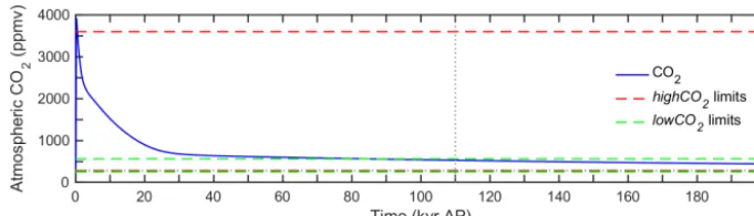
re-Figure 1.Time series of atmospheric CO2concentration (ppmv) for the next 200 kyr following logistic CO2emissions of 10 000 Pg C, run using thecGENIE model (Lord et al., 2016). Also shown are the upper and lower CO2limits of thehighCO2(red dashed lines) andlowCO2
(green dashed lines) ensembles. The pre-industrial CO2concentration of 280 ppmv (horizontal grey dotted line) and the 110 kyr AP cut-off for the high-CO2ensemble (vertical grey dotted line) are included for reference.
lease. To put this into perspective: current estimates of fossil fuel reserves are approximately 1000 Pg C, with an estimated ∼4000 Pg C in fossil fuel resources that may be extractable in the future (McGlade and Ekins, 2015), and up to 20– 25 000 Pg C in nonconventional resources such as methane clathrates (Rogner, 1997). The evolution of atmospheric CO2
concentration over the next 200 kyr for this emissions sce-nario is shown in Fig. 1. Although in thecGENIE simulation, atmospheric CO2 reaches a maximum of 3900 ppmv (parts
per million) within the first few hundred years, this concen-tration is not at equilibrium and only lasts for a couple of decades before decreasing. As a result, the concentration at 500 years into the experiment, 3600 ppmv, is chosen as the upper CO2 limit, which means that the climatic effects of
emissions of more than 10 000 Pg C cannot be estimated with the emulator.
By the end of the 1 Myr emissions scenario, atmospheric CO2 concentrations have nearly declined to pre-industrial
levels, reaching 285 ppmv. However, this experiment does not account for natural variations in the carbon cycle, which result in periodic fluctuations in CO2. For example, during
the Holocene (11 kyr BP to ∼1750 CE) atmospheric CO2
varied between 260 and 280 ppmv (Monnin et al., 2004). A value of 250 ppmv is therefore deemed to be appropriate to account for these natural variations in an unglaciated world, in addition to possible uncertainties in the model, and hence is assumed as the value of the lower CO2limit in the
ensem-ble.
The orbital and CO2parameter ranges that have been
se-lected are also applicable to unglaciated periods during the late Pliocene, when atmospheric CO2 was estimated to be
higher than pre-industrial values (Martinez-Boti et al., 2015; Raymo et al., 1996). In this study, we do not consider or at-tempt to simulate past or future glacial episodes, which may be accompanied by larger continental ice sheets (see Sect. 7 for more discussion), although the conditions required to ini-tiate the next glaciation, and extending the ensemble of GCM simulations to represent glacial states, are being investigated in a forthcoming study. The underlying assumption of our en-semble is that it is suitable for simulating periods for which
the CO2concentration is high enough to prevent entry into a
glacial state.
Two ensembles were generated, each made up of 40 sim-ulations, meeting the recommended 10 experiments per in-put parameter (Loeppky et al., 2009). One ensemble includes orbital values suitable for the next 1 Myr and a relatively small range of lower CO2values, whereas the other
ensem-ble represents the shorter-term future with a reduced range of orbital values and a larger range of higher CO2
concen-trations. This approach was adopted because various stud-ies have shown that on geological timescales of thousands to hundreds of thousands of years an emission of anthropogenic CO2 to the atmosphere is taken up by natural carbon cycle
processes over different timescales (Archer et al., 1997; Lord et al., 2016). A relatively large fraction of the CO2
perturba-tion is neutralised on shorter timescales of 103–104 years, but it takes 105–106years for atmospheric CO2
concentra-tions to very slowly return to pre-industrial levels (Colbourn et al., 2015; Lenton and Britton, 2006; Lord et al., 2016), if the effects of glacial–interglacial cycles and other natural variations, such as those due to imbalances between volcanic outgassing and weathering, are excluded. Hence, only a rel-atively short portion of the full million years has very high CO2 concentrations under any emissions scenario, with the
major part of the time having a CO2concentration no more
than several hundred parts per million by volume above pre-industrial, as demonstrated in Fig. 1.
The parameter ranges for the two ensembles, which are referred to as “highCO2” and “lowCO2”, are given in
Ta-ble 1. The cut-off point for thehighCO2ensemble is set at
110 kyr AP, as after this time eccentricity, which remained relatively low prior to this time, starts to increase more rapidly, and variability inesin$ andecos$ increases. This first ensemble therefore has CO2sampled up to 3600 ppmv,
and the orbital parameters are sampled within the reduced range of values that will occur over the next 110 kyr. The lowCO2 ensemble samples the full range of orbital values
and the upper CO2limit is set to 560 ppmv. This upper limit
also covers the range of CO2 concentrations that have been
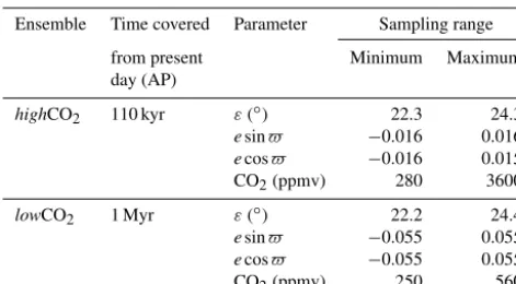
Table 1.Ensemble set-ups: sampling ranges for input parameters (obliquity,esin$,ecos$ and CO2) for thehighCO2andlowCO2
ensembles.
Ensemble Time covered Parameter Sampling range
from present Minimum Maximum day (AP)
highCO2 110 kyr ε(◦) 22.3 24.3 esin$ −0.016 0.016 ecos$ −0.016 0.015 CO2(ppmv) 280 3600 lowCO2 1 Myr ε(◦) 22.2 24.4 esin$ −0.055 0.055 ecos$ −0.055 0.055 CO2(ppmv) 250 560
2015; Seki et al., 2010). At 110 kyr AP in the 10 000 Pg C emissions scenario, the atmospheric CO2 concentration is
542 ppmv, which is rounded up to twice the pre-industrial at-mospheric CO2concentration (560 ppmv=2×280 ppmv), a
common scenario used in future climate-change modelling studies.
The benefits of the approach of having separate ensembles for high and low CO2mean that both parameter ranges have
sufficient sampling density, whilst also reducing the chance of unrealistic sets of parameters, in particular for the pe-riod of the next 110 kyr. During this time, CO2is likely to
be comparatively high, while eccentricity remains relatively low, andesin$ andecos$ exhibit relatively low variabil-ity. Having a separate ensemble in which CO2and the orbital
parameters are only sampled within the ranges experienced within the next 110 kyr avoids wasting computing time on pa-rameter combinations that are highly unlikely to occur, such as very high CO2and very high eccentricity. This
methodol-ogy also provides the additional benefit of the low-CO2
emu-lator being applicable to palaeo-modelling studies, as the en-semble encompasses an appropriate range of CO2and orbital
values for many past periods of interest, such as the Pliocene.
3.3 Generation of experiment ensembles
We used the Latin hypercube sampling function from the MATLAB Statistics and Machine Learning Toolbox (LHC; MATLAB, 2012) to generate the two ensembles, thereby effi-ciently sampling the four-dimensional input parameter space (Mckay et al., 1979). Briefly, this method divides the param-eter space within the prescribed ranges intonequally prob-able intervals, nbeing the number of experiments required, which in this case is 40 per ensemble.npoints are then se-lected for each input variable, one from each interval, with-out replacement. The sample points for the four variables are then randomly combined. The LHC sampling function also includes an option to maximise the minimum distance be-tween all pairs of points (the maxi–min criterion), which is
utilised here to ensure the set of experiments is optimally space filling.
For each ensemble, 3000 sample sets were created, with each set consisting of annbyp matrix,X, containing the four sampled input parameter values for each of the 40 ex-periments, and then the optimal sample set was selected as the final ensemble based on a number of criteria. Following Joseph and Hung (2008), we seek, in addition to the maxi-min criterion, to maximise det(XTX). Here, we will term this determinant the “orthogonality” because the columns of the design matrix will approach orthogonality as this deter-minant is maximised (assuming that input factors are nor-malised). However, a limitation of the method of sampling the parametersesin$ andecos$, rather than eccentricity and longitude of perihelion directly, is that due to the nature of theesin$ andecos$parameter space, the sampling pro-cess favours higher values of eccentricity over lower ones. This is not an issue for the longitude of perihelion because when eccentricity is low the value of this parameter has lit-tle effect on insolation. However, the value of obliquity se-lected for a given eccentricity value could have a signifi-cant impact on climate, meaning that it is desirable to have a relatively large range of obliquity values for low (<0.01) and high (>0.05) eccentricity values, in order to sample the boundaries sufficiently. It was observed that the sample sets with the highest orthogonality had comparatively few, if any, values of low eccentricity, also meaning that a very limited number of obliquity values were sampled for low eccentric-ity. We therefore adopted the approach whereby all sample sets that demonstrated normalised orthogonality values that were more than 1 SD (standard deviation) above the mean orthogonality were selected. From these, the single sample set with the greatest range of obliquity values for low ec-centricity, hence with maximal sampling coverage of the low-eccentricity boundary, was selected as the final ensem-ble design. The input parameter values for thehighCO2and
lowCO2ensembles are given in Table 2, and the distributions
in parameter space are illustrated in Fig. 2.
3.4 AOGCM simulations
The two CO2 ensembles were initially run with constant
modern-day GrIS and WAIS configurations (modice). All ex-periments were initiated from a pre-industrial spin-up exper-iment, with an atmospheric CO2concentration of 280 ppmv,
and pre-industrial ice sheet extents and orbital conditions. Atmospheric CO2 and the orbital parameters were kept
constant throughout each simulation, and each experiment was run for a total of 500 model years. This simulation length allows the experiments with lower CO2to reach
near-equilibrium at the surface. Experiments with higher CO2
have not yet equilibrated by the end of this period; the signif-icance of this is addressed in Sect. 3.6. A number of the very-high-CO2experiments caused the model to become unstable
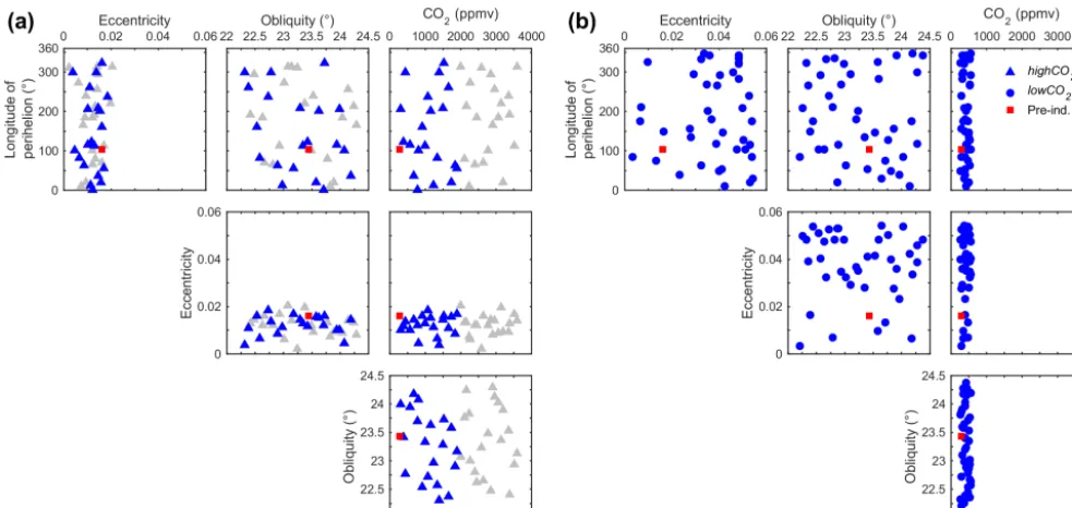
Figure 2.Distribution of 40 experiments produced by Latin hypercube sampling, displayed as two-dimensional projections through four-dimensional space.(a)highCO2ensemble and(b)lowCO2ensemble. The variables are eccentricity (e), longitude of perihelion ($,◦),
obliquity (ε,◦) and atmospheric CO2concentration (ppmv). A pre-industrial control simulation is shown in red. In thehighCO2ensemble,
experiments with CO2concentrations of more than 2000 ppmv, shown in grey, were excluded from the emulator.
Sect. 3.4 under “Very-high-CO2simulations”. A control
sim-ulation was also run for 500 years, with the atmospheric CO2
concentration and the orbital parameters set at pre-industrial values. All climate variable results for the model, unless specified, are an average of the final 50 years of the simu-lation. Anomalies compared with the pre-industrial control (i.e. emulated minus pre-industrial) are discussed and used in the emulator, rather than absolute values, to account for biases in the control climate of the model.
Very-high-CO2simulations
As mentioned previously, experiments in the highCO2
en-semble with CO2concentrations of greater than 3100 ppmv
become unstable. These experiments exhibit accelerating warming trends several hundred years into the simulation, which eventually cause the model to crash before comple-tion. This is the result of a runaway positive feedback in the GCM caused, at least in part, by the vertical distribution of ozone in the model being prescribed for modern-day cli-mate conditions. Consequently, the ozone distribution is not able to respond to changes in climate, meaning that when in-creased mean global temperatures result in an increase in al-titude of the tropopause and hence an extension of the tropo-sphere, relatively high concentrations of ozone, which were previously located in the stratosphere, enter the troposphere, resulting in runaway warming.
All other experiments ran for the full 500 years. However, those with a CO2concentration of 2000 ppmv or higher also
exhibited accelerating warming trends before the end of the simulation. Consequently, only simulations with CO2
con-centrations of less than 2000 ppmv (equivalent to a total CO2
release of up to 6000 Pg C) are included in the rest of this study, meaning the methodology is not appropriate for CO2
values greater than this. This equates to 20 experiments in total from thehighCO2ensemble, with CO2concentrations
ranging from 303 to 1901 ppmv. All 40 of thelowCO2
exper-iments were used.
3.5 Sensitivity to ice sheets
In addition to running the two ensembles with modern-day GrIS and WAIS configurations, we also investigated the cli-matic impact of reducing the sizes of the ice sheets. Many of the CO2values sampled, particularly in thehighCO2
ensem-ble, are significantly higher than pre-industrial levels, and if the resulting climate were to persist for a long period of time it could result in significant melting of the continental ice sheets over timescales of 103–104years (Charbit et al., 2008; Stone et al., 2010; Winkelmann et al., 2015).
We therefore set up thehighCO2andlowCO2ensembles
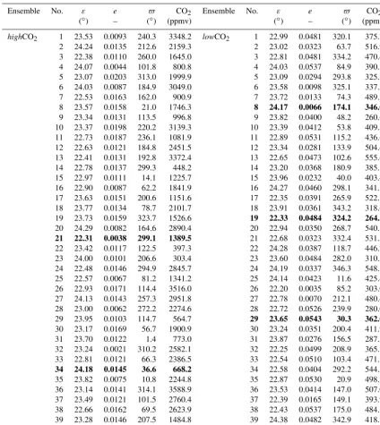
Table 2.Experiment set-up: orbital parameters (obliquity, eccentricity and longitude of perihelion) and atmospheric CO2concentration
for simulations in the highCO2 and lowCO2 ensembles. All experiments in both ensembles were run with modern ice sheet (modice)
configurations. Experiments shown in bold were also run with reduced ice sheet (lowice) configurations. The experiment number is given, and the experiment name is constructed using the ice sheet configuration, the ensemble name and the experiment number, for example, modice_lowCO2_1.
Ensemble No. ε e $ CO2 Ensemble No. ε e $ CO2 (◦) – (◦) (ppmv) (◦) – (◦) (ppmv)
highCO2 1 23.53 0.0093 240.3 3348.2 lowCO2 1 22.99 0.0481 320.1 375.7 2 24.24 0.0135 212.6 2159.3 2 23.02 0.0323 63.7 516.9 3 22.38 0.0110 260.0 1645.0 3 22.81 0.0481 334.2 470.4 4 24.07 0.0044 101.8 800.8 4 24.03 0.0537 84.9 390.3 5 23.07 0.0203 313.0 1999.9 5 23.09 0.0294 293.8 325.3 6 24.03 0.0087 184.9 3049.0 6 23.58 0.0098 325.1 337.5 7 22.53 0.0163 162.0 900.9 7 23.72 0.0133 74.3 489.2 8 23.57 0.0158 21.0 1746.3 8 24.17 0.0066 174.1 346.0
9 23.34 0.0131 113.5 996.8 9 23.82 0.0400 48.2 260.6 10 23.37 0.0198 220.2 3139.3 10 23.39 0.0412 53.8 409.5 11 22.73 0.0187 236.1 1081.9 11 22.89 0.0531 115.2 436.6 12 22.63 0.0121 184.8 2451.5 12 23.34 0.0281 133.9 504.4 13 22.41 0.0131 192.8 3372.4 13 22.65 0.0473 102.6 555.6 14 22.78 0.0137 299.3 448.2 14 23.20 0.0368 180.9 385.1 15 22.97 0.0111 14.1 1225.7 15 23.96 0.0232 40.0 403.4 16 22.90 0.0087 62.2 1841.9 16 24.27 0.0460 298.1 341.1 17 23.63 0.0151 200.6 1151.6 17 22.35 0.0391 265.9 522.1 18 23.77 0.0134 78.7 2101.7 18 23.91 0.0361 343.2 318.6 19 23.73 0.0159 323.7 1526.6 19 22.33 0.0484 324.2 264.5
20 24.29 0.0082 164.6 2890.4 20 22.94 0.0350 268.7 540.8
21 22.31 0.0038 299.1 1389.5 21 22.68 0.0323 332.4 531.5 22 23.42 0.0117 122.5 397.3 22 24.28 0.0387 118.7 446.7 23 24.00 0.0101 206.6 303.4 23 23.60 0.0484 282.0 310.5 24 22.48 0.0146 294.9 2845.7 24 24.19 0.0337 346.3 548.3 25 22.57 0.0067 81.2 1341.2 25 24.14 0.0423 11.6 425.4 26 22.93 0.0171 114.4 3516.0 26 22.20 0.0035 85.2 303.0 27 24.13 0.0143 257.3 2951.8 27 22.78 0.0070 212.1 480.4 28 23.00 0.0062 272.2 2274.6 28 22.72 0.0526 239.9 280.0 29 23.95 0.0103 114.7 564.7 29 23.65 0.0543 30.3 362.0
30 23.17 0.0169 56.7 1900.9 30 23.24 0.0351 200.4 411.9 31 23.70 0.0122 1.4 773.0 31 23.87 0.0276 156.5 287.5 32 23.24 0.0021 310.2 2582.1 32 22.25 0.0499 208.9 365.3 33 22.81 0.0121 66.3 2386.5 33 22.54 0.0510 103.4 471.1
34 24.18 0.0145 36.6 668.2 34 22.58 0.0404 292.2 544.5 35 23.82 0.0075 10.8 2244.8 35 22.87 0.0530 20.9 498.2 36 23.14 0.0141 314.1 3588.9 36 23.53 0.0414 147.0 507.0 37 23.49 0.0121 101.5 2760.4 37 22.39 0.0165 149.1 393.9 38 22.66 0.0162 69.5 2623.9 38 22.43 0.0537 175.0 484.8 39 23.28 0.0146 207.5 1484.8 39 24.38 0.0482 342.9 418.3 40 23.89 0.0092 21.1 3188.8 40 23.76 0.0504 127.0 528.1
de Wolde, 1999; Ridley et al., 2005; Stone et al., 2010) and WAIS (Huybrechts and de Wolde, 1999; Winkelmann et al., 2015), equivalent to ∼7 m (Ridley et al., 2005) and ∼3 m (Bamber et al., 2009; Feldmann and Levermann, 2015) of global sea level rise, respectively. Large regions of the EAIS show minimal changes or slightly increased surface eleva-tion, although there is substantial loss of ice in the Wilkes and Aurora subglacial basins (Haywood et al., 2016).
The same CO2 and orbital parameter sample sets were
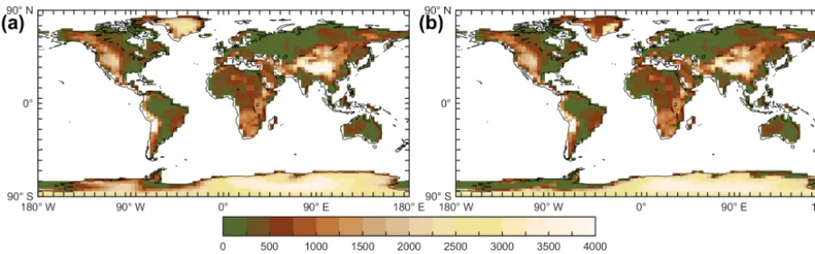
Figure 3.Orography (m) in the two ice sheet configuration ensembles:(a)modiceensemble and(b)lowiceensemble. Differences only occur over Greenland and Antarctica.
PRISM4 data, as well as the orography of any grid boxes that are projected to be ice-free. Soil properties, land surface type and snow cover were also updated for these grid boxes. Figure 3 compares the orography for themodiceandlowice ensembles, clearly showing the reduced extents for the ice sheets.
Pattern scaling of reduced ice simulations
It was expected that reducing the size of the continental ice sheets would have a relatively localised impact on climate (Lunt et al., 2004) and that the effect would be of a lin-ear nature. Therefore, a subset of five simulations from the two ensembles were selected as reduced ice sheet simula-tions (lowCO2– experiments 8, 19 and 29;highCO2–
exper-iments 21, and 34; see Table 2), covering a range of orbital and CO2values.
A comparison of the mean annual SAT anomaly for the five experiments showed that the largest temperature changes occur over Greenland and Antarctica, particularly in regions where there is ice in the modiceensemble but that are ice free inlowice. The spatial pattern of the change is also fairly similar across the simulations, suggesting that the response of climate to the extents of the ice sheets is largely inde-pendent of orbital variations or CO2concentration. The SAT
anomaly for the fivelowiceexperiments compared with their modiceequivalents was calculated and then averaged across the experiments, shown in Fig. 4a. The largest SAT anoma-lies occur locally to the GrIS and Antarctic ice sheet (AIS), accompanied by smaller anomalies in some of the surround-ing ocean regions (e.g. Barents and Ross seas), with no sig-nificant changes in SAT elsewhere, in line with the results of Lunt et al. (2004), Toniazzo et al. (2004) and Ridley et al. (2005). This SAT anomaly, caused by the reduced extents of the GrIS and WAIS, was then applied (added) to the mean annual SAT anomaly data for all otherhighCO2andlowCO2
modiceexperiments to generate the SAT data for twolowice ensembles.
Also shown in Fig. 4, for comparison, are mean annual SAT anomalies produced by the other forcings, including a doubling of CO2, the difference between maximum and
minimum obliquity and the difference between “warm” or-bital conditions and “cold” oror-bital conditions. The warm-ing caused by increased CO2is more widespread (Fig. 4b),
with the largest warming occurring at high latitudes and for land regions, in agreement with typical future-climate simu-lations (IPCC, 2013, p. 1059). The temperature change due to obliquity and warm versus cold orbital conditions is less than that for either reduced ice (compared to pre-industrial) or increased CO2. Changes in obliquity have the largest
im-pact on temperatures in high-latitude regions since the expo-sure of these regions to the sun’s radiation is most affected by changes in obliquity. Smaller temperature anomalies are ob-served over northern Africa and India and, since an increase in obliquity is indeed known to boost monsoon dynamics (e.g. Araya-Melo et al., 2015; Bosmans et al., 2015), changes in soil latent heat exchanges are therefore expected to con-tribute negatively to the temperature response. The compari-son of warm versus cold orbital conditions, which highlights (annual mean) temperature changes primarily caused by pre-cession, generally shows a warming trend, with the largest temperature changes occurring in monsoonal regions. Lower temperatures are observed in the Northern Hemisphere over northern Africa, India and East Asia, whilst warmer tempera-tures occur in the Southern Hemisphere over South America, southern Africa and Australia. Figure 4 demonstrates that the temperature forcing caused by CO2affects mean annual
tem-peratures on a global scale, whilst the forcing due to ice sheet and orbital changes affects mean annual temperatures in spe-cific regions, having a limited impact on global mean temper-atures. This is supported by the relatively high global mean SAT anomaly for the 2×CO2scenario of 4.2◦C, compared
Figure 4.Mean annual SAT (◦C) anomalies produced by the various climate forcings.(a)Thelowiceexperiments compared with their
modiceequivalents, averaged across the fivelowiceexperiments.(b)–(d)Idealised experiments performed using themodiceemulator. All orbital and CO2conditions are set to pre-industrial values unless specified:(b)2×pre-industrial CO2,(c)maximum obliquity compared
to minimum obliquity,(d)warm orbital conditions (high eccentricity, NH summer at perihelion) compared to cold orbital conditions (low eccentricity, NH summer at aphelion). The different forcings result in global mean SAT anomalies of(b)4.2◦C,(c)0.4◦C and(d)0.4◦C.
3.6 Calculation of equilibrated climate
Given the high values of CO2concentration in many of the
experiments, particularly in thehighCO2ensemble, even by
the end of the 500-year running period the climate has not yet reached steady state. We therefore estimated the fully equili-brated climate response using the methods described below.
3.6.1 Gregory plots
In order to estimate the equilibrated response, we applied the method of Gregory et al. (2004) to the model results, regress-ing the net radiative flux at the top of the atmosphere (TOA) against the global average SAT change, as displayed in fig-ures termed Gregory plots (Andrews et al., 2012, 2015; Gre-gory et al., 2015). In this method, for an experiment that has a constant forcing applied (i.e. with no inter-annual variation) it can be assumed that
N =F−α1T , (16)
where N is the change in the global mean net TOA ra-diative flux (W m−2), F is the effective radiative forcing
(W m−2, positive downwards),αis the climate feedback
pa-rameter (W m−2◦C−1) and 1T is the global mean annual
SAT change compared with the control simulation (◦C). This method works on the assumption that ifF andα are con-stant,N is an approximately linear function of1T. By lin-early regressing1T againstN, bothF (intercept of the line at 1T=0) and −α (slope of the line) can be diagnosed. The intercept of the line atN=0 provides an estimate of the equilibrium SAT change (relative to the pre-industrial SAT) for the experiment, denoted1Teqg to indicate it was
calcu-lated from the Gregory plots, and is equal toF /α. This is in contrast to the SAT change calculated directly from the GCM model data by averaging the final 50 years of the ex-periment (1T500).
The Gregory plots for two modice experi-ments, modice_lowCO2_13 (CO2 555.6 ppmv) and
modice_highCO2_17 (CO2 1151.6 ppmv), are shown
in Fig. 5. These experiments were selected as they have CO2 values nearest to the 2× and 4× pre-industrial CO2
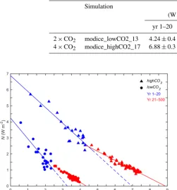
Table 3.Parameter values estimated from Gregory plots for the 2×and 4×pre-industrial CO2simulations. Shown are the effective radiative
forcing (F, W m−2) and the climate feedback parameter (α, W m−2◦C−1) for years 1–20 and 21–100. The uncertainties are the standard error from the linear regression.
Simulation F α
(W m−2) (W m−2◦C−1) yr 1–20 yr 21–100 yr 1–20 yr 21–100 2×CO2 modice_lowCO2_13 4.24±0.4 – −1.30±0.2 −0.68±0.05
4×CO2 modice_highCO2_17 6.88±0.3 – −0.99±0.1 −0.56±0.02
Figure 5. Gregory plot showing change in TOA net down-ward radiation flux (N, W m−2) as a function of change in global mean annual SAT (1T, ◦C) for approximate 2×CO2
(modice_lowCO2_13, circles) and 4×CO2(modice_highCO2_17, triangles) experiments. Lines show regression fits to the global mean annual data points for years 1–20 (blue) and years 21–500 (red). Data points are mean annual data for years 1–20 (blue) and mean decadal data for years 21–500 (red). The1T intercepts (N=0) of the red lines give the estimated equilibrated SAT (1Teqg)
for the two experiments. The1T intercepts of the dashed blue lines represent the equilibrium that the experiment would have reached if the feedback strengths in the first 20 years had been maintained. SAT is shown as an anomaly compared with the pre-industrial con-trol simulation.
data for years 21–500. The regression fits are to mean annual data in each case, and years 1–20 and 21–500 were fitted separately. The values for F and α estimated from Fig. 5 are presented in Table 3. These values are slightly lower than those identified in other studies using the same method. For example, Gregory et al. (2004) used HadCM3 to run experiments with 2×and 4×CO2, obtaining values
for years 1–90 of 3.9±0.2 and 7.5±0.3 W m−2 for F, and −1.26±0.09 and −1.19±0.07 W m−2◦C−1 for α, respectively. Andrews et al. (2015) calculated F to be 7.73±0.26 W m−2 and α to be −1.25 W m−2◦C−1 for years 1–20 and −0.74 W m−2◦C−1 for years 21–100 for 4×CO2 simulations using HadCM3. The differences
between our results and theirs may be due to the fact that we used MOSES2.1 and the TRIFFID vegetation model, whereas they used MOSES1, which is a different land-surface scheme and does not account for vegetation feedbacks.
The decrease in the climate response parameter (α) as the experiment progresses suggests that the strength of the cli-mate feedbacks changes as the clicli-mate evolves over time. Consequently, the1T intercept (N=0) for the first 20 years of the simulation underestimates the actual warming of the model. Over longer timescales, the slope of the regression line becomes less negative, implying that the sensitivity of the climate system to the forcing increases (Andrews et al., 2015; Gregory et al., 2004; Knutti and Rugenstein, 2015). This non-linearity has been found to be particularly apparent in cloud feedback parameters, in particular shortwave cloud feedback processes (Andrews et al., 2012, 2015). A number of studies have attributed this strengthening of the feedbacks to changes in the pattern of surface warming (Williams et al., 2008), mainly in the eastern tropical Pacific where an in-tensification of warming can occur after a few decades, but also in other regions such as the Southern Ocean (Andrews et al., 2015). The impact of variations in ocean heat uptake has also been suggested to be a contributing factor (Geoffroy et al., 2013; Held et al., 2010; Winton et al., 2010).
We take the1T intercept (N=0) for years 21–500 to give the equilibrium temperature change (1Teqg) for the
experi-ments, equating to values of 4.3 and 8.9◦C for the 2×and 4×CO2 scenarios in Fig. 5. A limitation of this approach
is that it assumes that the response of climate to a forcing is linear after the first 20 years, which has been shown to be unlikely in longer simulations of several decades or cen-turies (Andrews et al., 2015; Armour et al., 2013; Winton et al., 2010). However, a comparison of the difference in tem-perature response to upper- and deep-ocean heat uptake and its contribution to the relationship between net radiative flux change (N) and global temperature change (1T) in Geof-froy et al. (2013) indicated that the method of Gregory et al. (2004) of fitting two separate linear models to the early and subsequent (N,1T) data gives a good approximation of 1Teqg,F andαas they have been calculated here. A study
ac-Figure 6.Equilibrated global mean annual change in SAT (1Teqg, ◦
C) estimated using the methodology of Gregory et al. (2004) against global mean annual change in SAT (1T500,◦C) at year 500
(average of final 50 years) for thelowCO2(circles) andhighCO2 (triangles)modiceensembles. The colours of the points indicate the CO2concentration of the experiment, from low (blue) to high (yel-low). The 1 : 1 line (dashed) is included for reference. SAT is shown as an anomaly compared with the pre-industrial control simulation.
tual value, obtained by running the simulation very close to equilibrium (∼6000 years). However, this was using the ECHAM5/MPIOM model, meaning that it is not necessarily also true for HadCM3.
Given that the slope of the 21–500 years regression line ap-pears to become shallower with time, the estimates of1Teqg
should be taken as a lower limit of the actual equilibrated SAT anomaly. However, this tendency to flatten, particularly as the CO2 concentration is increased, further justifies our
use of the Gregory methodology; by the end of 500 years the high-CO2experiments have not yet reached steady state,
and even in the lower-CO2experiments SAT increases very
slowly and will thus likely take a long time to reach equi-librium. It would therefore not be feasible to run most of these experiments to steady state using a GCM, due to the as-sociated computational and time requirements. Furthermore, on longer timescales the boundary conditions (orbital charac-teristics and, more importantly, atmospheric CO2
concentra-tions) would have changed, such that, in reality, equilibrium would never be attained.
3.6.2 Equilibrated climate
The final estimates of 1Teqg for the lowCO2 andhighCO2
modiceensembles range from a minimum of−0.4◦C (CO2
264.5 ppmv) to a maximum of 12.5◦C (CO21900.9 ppmv).
Figure 6 illustrates the difference between global mean annual SAT anomaly calculated from the GCM model
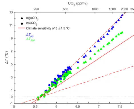
Figure 7.Equilibrated global mean annual change in SAT (1Teq,
◦C, blue), estimated by applying the1Tg
eq/1T500ratio identified
using the Gregory methodology to the GCM data, against atmo-spheric CO2(ppmv) for thelowCO2(circles) andhighCO2
(trian-gles)modiceensembles. Also shown is1T500(green), along with the idealised relationship between ln(CO2) and1T (red lines) for a
climate sensitivity of 3◦C (solid), 1.5◦C (lower dashed) and 4.5◦C (upper dashed) (IPCC, 2013). SAT is shown as an anomaly com-pared with the pre-industrial control simulation.
data (1T500) and calculated using the Gregory plot (1Teqg).
Experiments with CO2 below or near pre-industrial levels
tended to reach equilibrium by the end of the 500 years, mak-ing a Gregory plot unnecessary; hence,1Teqg is taken to be
the same as1T500in these cases. As CO2increases, the data
points in Fig. 6 deviate further from the 1 : 1 line. This is the result of the ratio between1Teqg and1T500increasing, as the
experiments grow increasingly far from equilibrium by the end of the GCM run with increasing CO2.
We next calculated the ratio between1Teqg and1T500for
each experiment (1Teqg/1T500), which represents the
frac-tional increase in climate change still due to occur after the end of the 500-year model run in order for steady state to be reached. To estimate the fully equilibrated climate anomaly, the spatial distribution of mean annual SAT anomaly was multiplied by the1Teqg/1T500ratio. The ratio identified for
each experiment is assumed to be equally applicable to all grid boxes. The same scaling ratio was also applied to the precipitation anomaly data to estimate the equilibrated mean annual precipitation.
The equilibrated global mean annual SAT anomaly (1Teq)
for the highCO2 andlowCO2 modice ensembles is plotted
against ln(CO2) in Fig. 7, along with1T500 for reference.
Also plotted in Fig. 7 are a number of lines illustrating ide-alised relationships between1Teqand CO2based on a range
sensitiv-ity is 1.5 to 4.5◦C (IPCC, 2013), hence sensitivities of 1.5, 3 and 4.5◦C have been plotted. The size of the correction required to calculate 1Teq from 1T500 increases with
in-creasing CO2 and brings the final temperature estimates in
line with the expected response (red lines), further increas-ing our confidence. The1Teqestimated for the experiments
generally follows the upper line, equivalent to an equilib-rium climate sensitivity of 4.5◦C, which is higher than a previous estimate of 3.3◦C for HadCM3 (Williams et al., 2001). This difference may be due to our simulations be-ing “fully equilibrated” followbe-ing the application of the Gre-gory plot methodology. In addition, Williams et al. (2001) used an older version of HadCM3 and prescribed vegetation (MOSES1), whilst in this study interactive vegetation is used (MOSES2.1 with TRIFFID).
4 Calibration and evaluation of the emulator
By considering different contributions of modern and low ice, high and low CO2, different number of PCs, and
dif-ferent values for the correlation length hyperparameters, we generated an ensemble of emulators, in order to test their rel-ative performance. The modiceandlowice ensembles were treated as independent data sets that were used separately when calibrating the emulator since ice extent is not defined explicitly as an input parameter in the emulator code. This approach was adopted, rather than including the ice sheet ex-tent as an active input parameter to the emulator, because only two ice sheet configurations have been simulated, which are not sufficient for an interpolation. One of the main bene-fits of including ice sheet extent as an active input parameter would be to emulate changing ice sheets over time, but this was beyond the scope of this study. ln(CO2) was used as one
of the four input parameters, along with obliquity, esin$ andecos$. The performance of each emulator was assessed using a leave-one-out cross-validation approach, in which a series of emulators is constructed and used to predict one left-out experiment each time. For example, for thelowCO2
modiceensemble (40 experiments), 40 emulators were cali-brated with one experiment left out of each. This left-out ex-periment was then reproduced using the corresponding em-ulator and the results were compared with the actual experi-ment results. The number of grid boxes for each experiexperi-ment calculated to lie within different standard deviation bands, and the RMSEs averaged across all the emulators were used as performance indicators to compare the different input con-figurations and hyperparameter value selections. The results in this section are applicable to themodiceemulator, unless otherwise specified; however, the calibration and evaluation for thelowiceemulator yielded similar trends and results.
4.1 Sensitivity to input data
We investigated the impact on performance of calibrating the emulator on the highCO2 andlowCO2 modice
ensem-bles separately and combined. ThelowCO2modiceemulator
generally performs slightly better in the leave-one-out cross-validation exercise than thehighCO2modiceversion, with a
lower RMSE and fewer grid boxes with an error of more than 2 SD. Combining the two ensembles into one emulator re-sults in a similar RMSE to thelowCO2-onlymodiceemulator
but decreases the RMSE compared with thehighCO2-only
modiceemulator. As a consequence, we took the approach of calibrating the emulator on the combined ensembles for the rest of the study. This has the advantage that continuous sim-ulations of climate with CO2levels that cross the boundary
between the high- and low-CO2 ensembles (∼560 ppmv),
such as may be appropriate for emulation of future climate, can be performed using one emulator, rather than having to calibrate separate emulators for different time periods based on CO2concentration. There is also no loss of performance
in the emulator for either set of CO2ranges, but rather a slight
improvement for thehighCO2ensemble.
4.2 Optimisation of hyperparameters
We calibrated two separate emulators, the first using the modice data and the second using the lowice data, both with 60 experiments each (combinedhighCO2andlowCO2).
The input factors (ε, esin$, ecos$ and ln(CO2)) were
standardised prior to the calibration being performed; each was centred in relation to its column mean, and then scaled based on the standard deviation of the column. We tested different emulator configurations by varying the number of PCs retained, ranging from 5 to 20, and for each emulator configuration, the correlation length scalesδ and nuggetν were optimized by maximisation of the penalised likelihood. This optimisation was carried out in log space, ensuring that the optimized hyperparameters would be positive. A leave-one-out validation was performed each time, and the modiceandlowiceconfigurations that performed best were selected as the final two optimized emulators. We found that amodiceemulator retaining 13 PCs has the lowest RMSE and a relatively low percentage of grid boxes with errors of more than 2 SD. The scalesδ for the modice emulator are 7.509 (ε), 3.361 (esin$), 3.799 (ecos$), and 0.881 (CO2)
and the nugget is 0.0631. In contrast, alowiceemulator using 15 principal components exhibits the best performance, with length scalesδof 5.597 (ε), 2.887 (esin$), 3.273 (ecos$), and 0.846 (CO2) and a nugget of 0.0925. In both cases, the
scales for the three orbital parameters are larger than the range associated with the input factors, indicating that the response is relatively linear with respect to these terms.
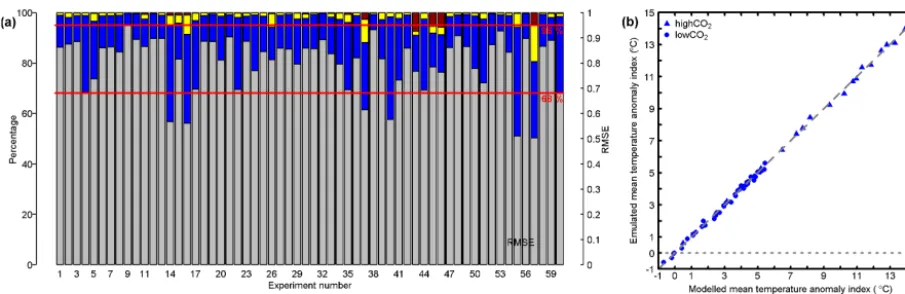
Figure 8.Evaluation of emulator performance.(a)Bars give the percentage of grid boxes for which the emulator predicts the SAT of the left-out experiment to within 1, 2, 3 and more than 3 SD (standard deviations). Also shown is the RMSE for the experiments (black circles). Red lines indicate 68 and 95 %.(b)Global mean annual SAT index (◦C) calculated by the emulator and the GCM for thelowCO2(circles)
andhighCO2(triangles)modiceensembles. The 1 : 1 line (dashed) is included for reference. Note: this is the mean value for the GCM output
data grid assuming all grid boxes are of equal size, hence not taking into account variations in grid box area: we therefore refer to it as a SAT index. SAT is shown as an anomaly compared with the pre-industrial control simulation.
which roughly corresponds to the 68 and 95 % ratios ex-pected for a normal distribution, suggesting that the uncer-tainty in the prediction is being correctly captured.
Several of the experiments performed considerably worse than others, exhibiting below the expected number of grid boxes with errors within 1 SD (for reference, the mean value for 1 SD across the left-out experiments is 0.3◦C), and/or higher than the expected number of grid boxes with errors of greater than 2 SD, which is generally accompa-nied by a higher RMSE. However, the input conditions for these experiments are not particularly similar or unique. Ex-periments modice_highCO2_43, modice_highCO2_45 and modice_highCO2_46 all have a fairly low eccentricity and obliquity and a CO2concentration of∼1000 ppmv, but there
are multiple experiments with similar values that have lower RMSE values. A spatial map of the errors (not shown) in-dicates that the grid boxes with errors of 3 or more standard deviations are at high northern latitudes in these experiments. However, the signs of the anomalies are not the same across these experiments, as the emulator overestimates the Arctic SAT anomaly in modice_highCO2_43 and underestimates it in modice_highCO2_45 and modice_highCO2_46. This sug-gests that the emulator is perhaps not quite capturing the full model behaviour in high northern latitudes, particularly for low eccentricity values, but this is certainly not true for all experiments. The errors in the experiments are generally less than±4◦C, and for most of the Arctic much lower than that. Note that the Arctic is a region in the model with high inter-annual variability; thus, one factor may be that the model simulations that are used to calibrate the emulator are not representative of the true stationary mean. There does not ap-pear to be any obvious systematic error associated with the input parameters, suggesting that errors are less likely to be an issue resulting from the design of the emulator and more
likely to arise from run-to-run variability in the behaviour of the underlying GCM.
Figure 8b compares the mean annual “SAT index” for each left-out experiment calculated by the GCM and the corre-sponding emulator (note: this is the mean value for the GCM output data grid assuming all grid boxes are of equal size, hence not taking into account grid box area). There are no ob-vious outliers, and the emulated means are relatively close to their modelled equivalents. There also does not appear to be any significant loss of performance at very low or very high temperature, and therefore at very low or very high CO2.
In summary, our calibration and evaluation shows that the emulator is able to reproduce the left-out ensemble simula-tions reasonably well, with no obvious systematic errors in its predictions. Using the emulator, calibrated on the full set of 60 simulations (modiceor lowice), we are able to simu-late global climate development over long periods of time (several hundred thousand years or longer). Provided that the atmospheric CO2 levels for the period are known and are
within the limits of those used to calibrate the emulator, ice sheets do not change outside of the two configurations con-sidered in the two ensembles, and the topography and land– sea mask are unchanged.
In the next two sections, we present illustrative examples of a number of potential applications of the emulator by ap-plying it to the late Pliocene in Sect. 5 and the next 200 kyr in Sect. 6.
5 Application of the emulator to the late Pliocene
Table 4. Mean temperature anomalies and uncertainties (1 SD – standard deviation) for the period 3300–2800 kyr BP estimated by the emulator and alkenone proxy data for the four ODP/IODP sites.
ODP/IODP Location Emulated SAT anomaly Proxy data SST anomaly
site (◦C) (◦C)
Lat Long 280 ppmv 350 ppmv 400 ppmv Prahl et al. Muller et al. (1988) (1998) 9821 North Atlantic 57.5◦N 15.9◦W 0.6±0.4 2.4±0.3 3.3±0.3 5.4 5.7 U13132 North Atlantic 41.0◦N 33.0◦W −0.8±0.3 0.0±0.2 0.8±0.2 1.6 2.0 7223 Arabian Sea 16.6◦N 59.8◦E 0.0±0.2 1.0±0.2 1.7±0.2 1.0 1.7 6623 Tropical Atlantic 1.4◦S 11.7◦W 0.2±0.2 0.9±0.2 1.3±0.2 1.3 1.9
1Lawrence et al. (2009).2Naafs et al. (2010).3Herbert et al. (2010).
To illustrate this, we applied thelowiceemulator to the late Pliocene and compared the results to palaeo-proxy data for the period. The lowice emulator was used because the ice sheets in this configuration are the PRISM4 Pliocene ice sheets (Dowsett et al., 2016). It should be noted, however, that this approach is only appropriate for periods of the Pliocene with equivalent or less-than-modern ice sheet ex-tents (i.e. not glacial conditions), and that palaeogeographic changes for the Pliocene are not included here (see Sect. 7 for further discussion). We also tested themodiceemulator, which, in agreement with the findings in Sect. 4, had a lim-ited impact on the long-term evolution of global sea surface temperatures (SSTs) outside the immediate region of the ice sheets themselves. Potential applications of the emulator for palaeoclimate are described below.
5.1 Time series data
One application of the emulator is to produce a time se-ries of the continuous evolution of climate for a particu-lar time period, as is illustrated here where climate is sim-ulated at 1 kyr intervals over the period 3300–2800 kyr BP. This period of the late Pliocene was selected because it has been extensively studied as part of a number of projects (e.g. PRISM; Dowsett et al., 2016; Dowsett, 2007, PlioMIP; Haywood et al., 2010, 2016), represents the warm phase of climate (interglacial conditions) and does not include ma-jor glaciations – though the M2 cooling event may persist to the very start of the simulation at 3300 kyr BP, and the simulated period does include periods of likely glaciation, such as KM2 (∼3100 kyr BP) and G20 (∼3000 kyr BP). The emulator would not be appropriate for periods of extensive glaciation and may not be well-matched to the periods of lesser glaciation included within the simulated interval. Or-bital data for each 1 kyr (Laskar et al., 2004) were provided as input to the calibrated emulator, along with three repre-sentative CO2concentrations. Three CO2reference scenarios
were initially emulated, with constant concentrations of 280, 350 and 400 ppmv (although note that in reality, CO2varied
on orbital timescales during this period; Martinez-Boti et al., 2015).
To illustrate the comparison of the emulator results to palaeo-proxy data, SST data for various locations were com-pared with the emulated SAT for the equivalent grid box. Specifically, alkenone-derived palaeo-SST estimates from four (Integrated) Ocean Drilling Program (IODP/ODP) sites were used: ODP Site 982 (North Atlantic; Lawrence et al., 2009), IODP Site U1313 (North Atlantic; Naafs et al., 2010), ODP Site 722 (Arabian Sea; Herbert et al., 2010) and ODP Site 662 (tropical Atlantic; Herbert et al., 2010). The loca-tions of the sites are shown in Fig. 9a and detailed in Table 4. These Pliocene datasets were selected because they are all of sufficiently high resolution (≤4 kyr) for the impacts of indi-vidual orbital cycles on climate to be captured, whilst cov-ering a range of locations and climatic conditions. Alkenone data are shown converted to SST using two commonly ap-plied calibrations: Prahl et al. (1988) and Muller et al. (1998). All temperatures are presented as an anomaly compared with pre-industrial. The emulator results are compared with the SAT for the relevant grid box in the pre-industrial control ex-periment, whilst the proxy data are compared with SST ob-servations for the relevant location taken from the HadISST data set (Rayner et al., 2003). Observations are annual means and are averaged over the period 1870–1900 CE.
Table 4 presents the mean SAT anomaly (compared with pre-industrial) for the modelled period as estimated by the emulator for the 280 ppmv scenario for each of the four grid boxes. The mean increases with increasing CO2, by ∼1◦C
at low latitudes to 2–3◦C at high latitudes for atmospheric CO2 of 400 ppmv. Figure 10 illustrates the evolution of
an-nual mean temperature variations through the late Pliocene as calculated using the various methods. For the equatorial and Arabian Sea sites (662 and 722), the SAT and SST es-timates are relatively similar to each other in terms of the general estimated temperature, particularly for the higher-CO2scenarios of 350 and 400 ppmv. However, the