www.ocean-sci.net/4/275/2008/
© Author(s) 2008. This work is distributed under the Creative Commons Attribution 3.0 License.
Ocean Science
Mutually consistent thermodynamic potentials for fluid water, ice
and seawater: a new standard for oceanography
R. Feistel1, D. G. Wright2, K. Miyagawa3, A. H. Harvey4, J. Hruby5, D. R. Jackett6, T. J. McDougall6, and W. Wagner7 1Leibniz Institute for Baltic Sea Research, 18119 Warnem¨unde, Germany
2Bedford Institute of Oceanography, Dartmouth, NS, Canada 34-12-11-628, Nishiogu, Arakawa-ku, Tokyo 116-0011, Japan
4National Institute of Standards and Technology, Boulder, CO 80305, USA 5Institute of Thermomechanics of the ASCR, v.v.i., Prague, Czech Republic
6Centre for Australian Weather and Climate Research: A partnership between CSIRO and the Bureau of Meteorology,
Hobart, TAS, Australia
7Ruhr-Universit¨at Bochum, 44780 Bochum, Germany
Received: 5 June 2008 – Published in Ocean Sci. Discuss.: 11 July 2008
Revised: 29 October 2008 – Accepted: 18 November 2008 – Published: 12 December 2008
Abstract. A new seawater standard for oceanographic and engineering applications has been developed that consists of three independent thermodynamic potential functions, de-rived from extensive distinct sets of very accurate experimen-tal data. The results have been formulated as Releases of the International Association for the Properties of Water and Steam, IAPWS (1996, 2006, 2008) and are expected to be adopted internationally by other organizations in subsequent years. In order to successfully perform computations such as phase equilibria from combinations of these potential func-tions, mutual compatibility and consistency of these indepen-dent mathematical functions must be ensured. In this article, a brief review of their separate development and ranges of validity is given. We analyse background details on the con-ditions specified at their reference states, the triple point and the standard ocean state, to ensure the mutual consistency of the different formulations, and the necessity and possi-bility of numerically evaluating metastable states of liquid water. Computed from this formulation in quadruple pre-cision (128-bit floating point numbers), tables of numerical reference values are provided as anchor points for the con-sistent incorporation of additional potential functions in the future, and as unambiguous benchmarks to be used in the determination of numerical uncertainty estimates of double-precision implementations on different platforms that may be customized for special purposes.
Correspondence to: R. Feistel ([email protected])
1 Introduction
The International Equation of State of Seawater (EOS-80, Fofonoff and Millard 1983) has successfully served the needs of oceanographers for three decades. Challenged by cli-mate change, equipped with more powerful computers, and confronted with new and more accurate standards in related fields of science and technology, the SCOR/IAPSO Work-ing Group 127 (WG127) was established and charged with developing a new seawater standard for oceanography.
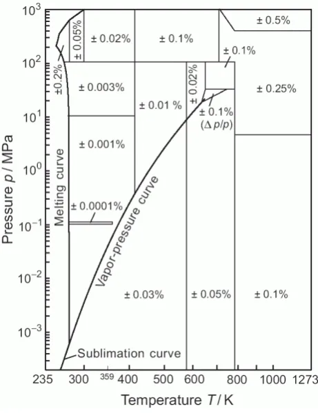
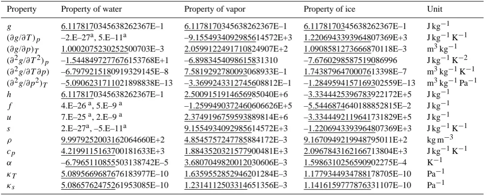
Fig. 1. Range of validity (excluding the ice phases at the left border line) and uncertainty of water density in the IAPWS-95 formulation.
water is already transformed into ice or vapor. A discussion of this work is presented in Sect. 4.
The presence of sea salt in water changes water’s thermo-dynamic properties. The saline part of a Gibbs potential of seawater (i.e., the addition to the Gibbs potential of pure wa-ter required to represent seawawa-ter) has now been dewa-termined for the quantitative description of these deviations (Feistel, 2003, 2008). For its application to seawater under extreme natural conditions or in technical systems such as desalina-tion plants, the range of validity of the saline Gibbs funcdesalina-tion has been extended to 80◦C and covers salinities extending from 0 to 120 g/kg, for which experimental data of adequate accuracy are available. The salinity range extends beyond the currently valid Practical Salinity Scale of 1978, PSS-78, at both low and high values. This problem is circumvented by using a new salinity scale termed Reference-Composition Salinity that was developed by WG127 (Millero et al., 2008). Saturation conditions for particular components of sea salt are discussed by Marion et al. (2008a, b).
The combination of the Helmholtz function for pure water, the Gibbs potential for salt-free ice and the saline part of the Gibbs potential provide the foundation for the computation of the thermodynamic properties of pure water and sea water within a new, unified and fully consistent framework.
Our approach of constructing a new seawater standard ex-plicitly from three distinct thermodynamic potential func-tions is unprecedented and has not been discussed in the sci-entific literature before. We discuss the conditions that need to be met to realize this novel approach as well as the so-lutions found to overcome the problems encountered. The ambiguities of different triple-point definitions and their im-plications for the formulation of seawater thermodynamics are analysed in Sect. 3. Revising earlier definitions (Feis-tel, 1993, 2003; Feistel and Hagen, 1995), the new WG127 specification of the seawater reference point is given and its properties are considered in detail in the same section.
In the appendix, highly accurate numerical values for the properties at the reference states of water and seawater are provided. In particular, we have recomputed the numeri-cal check values published in the Releases IAPWS-95 for fluid water, IAPWS-06 for ice and IAPWS-08 for seawater (IAPWS, 2008), using quadruple-precision calculations, and these are presented to 20 significant figures. These results provide unambiguous benchmarks against which double-precision implementations of the new seawater standard on different platforms can be validated.
In this paper, formula symbols are used which in some cases deviate from the common symbols used in oceanogra-phy. In particular,p is absolute pressure (in Pa, MPa, etc.) rather than sea pressure (relative top0=101 325 Pa), andwis sound speed (in m/s).SAis used to represent Absolute Salin-ity, which we note is not accurately represented by Practi-cal Salinity. For the relation between Absolute and PractiPracti-cal Salinity, see Millero et al. (2008).
2 Development of the formulations
In 1984, the International Association for the Properties of Steam (IAPS) adopted the Helmholtz potential developed by Haar et al. (1982, 1984) as the international standard some-times referred to as IAPS-84. At its 1990 meeting in Buenos Aires, IAPWS (the successor of IAPS) agreed on the need for a replacement of IAPS-84 which should be based on the ITS-90 temperature scale, represent a wider range of data, and better represent the critical and the metastable regions. This led to the approval of the Helmholtz function developed by Pruß and Wagner (1995) as the formulation IAPWS-95, which was adopted in its final form by IAPWS (1996) in Fredericia, Denmark, and is described in detail by Wagner and Pruß (2002). Its validity range in temperature and pres-sure is shown in Fig. 1. Fortran source code of an implemen-tation is available from the digital supplement of Feistel et al. (2008).
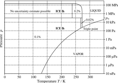
particular in compressibility. In a subsequent, more compre-hensive approach, the entire region of existence of ice Ih was covered by a new Gibbs function developed by Feistel and Wagner (2005). Its source code was published by Feistel et al. (2005) in the digital supplement. An improved version in-cluding additional data, in particular for the absolute entropy at the melting point (Feistel and Wagner, 2006), was adopted by IAPWS (2006) in Witney, UK. The range of validity of this formulation, which we will refer to as IAPWS-06, is shown in Fig. 2. Its source code with the updated coefficients is available from Feistel et al. (2008).
Ice Ih is the ice phase I that occurs under normal pres-sure and temperature conditions, in contrast to the ices II, III etc. which exist at very high pressures or low temperatures. Ice Ih possesses a stable hexagonal crystal lattice rather than a cubic one (termed ice Ic). The possibility of construct-ing Gibbs functions for the different high-pressure ice phases (>200 MPa) is discussed by Tchijov et al. (2008a, b).
The possibility of an extension in the form of a Gibbs func-tion for vapor below 130 K has recently been discussed by Feistel and Wagner (2007) and Riethmann et al. (2008) and will be implemented in the forthcoming source code library (Feistel et al., 2009; Wright et al., 2009).
More as a theoretical concept than a practical algo-rithm, a Gibbs function for seawater was described by Fo-fonoff (1962). During the development of the International Equation of State of Seawater (EOS-80), apparently no at-tempt was made to combine the theoretical concept with the available data to build such a thermodynamic potential, even though all necessary properties were quantitatively available before 1980. Separate correlation equations for the density, heat capacity, sound speed and freezing temperature were derived and adopted as the new standard for oceanography (Fofonoff and Millard, 1983), and they still remain as the in-ternational standard after nearly three decades.
Additional thermal and colligative properties published by Millero and Leung (1976) were used in combination with the EOS-80 equations for the construction of the first Gibbs function of seawater (Feistel, 1993). Feistel and Ha-gen (1995) improved this function by including additional data, e.g. for the sound speed and the temperatures of max-imum density, and conversion to ITS-90. Properties such as entropy and enthalpy that are available from this formulation in a consistent form are of growing interest for more accurate ocean models (McDougall, 2003; McDougall et al., 2003; Griffies et al., 2005; Jackett et al., 2006; Tailleux, 2008; Mc-Dougall et al., 2008).
After the appearance of the fundamental paper of Wag-ner and Pruß (2002), a systematic improvement of the Gibbs function of seawater proved possible by replacing pure-water properties of the Gibbs function of Feistel and Hagen (1995) by those computed from IAPWS-95 (Feistel, 2003). The re-lated source code for seawater can be found in the digital supplement of Feistel (2005), and with the same mathemati-cal structure but improved coefficients in Feistel et al. (2008).
0 50 100 150 200 250 300
10 nPa 1 µPa 100 µPa 10 mPa 1 Pa 100 Pa 10 kPa 1 MPa 100 MPa
P
re
ss
u
re
p
Temperature T / K
p0 Triple point
LIQUID
VAPOR No uncertainty estimate possible
0.1%
0.02% 0.2%
ICE Ih
ICE Ih
Fig. 2. Range of validity, shown in bold, and uncertainty of ice density in the IAPWS-06 formulation. The Gibbs function of ice remains valid at pressures even below the range shown here (it can be extrapolated to negative pressures to represent the effects of ten-sile stress), but the validity of IAPWS-95 for water vapor ends at T=130 K and hence does not extend belowp=10 nPa.
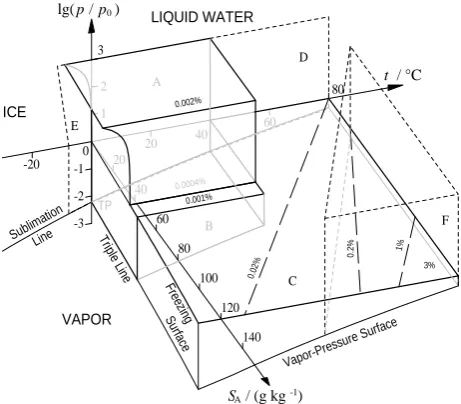
The 2008 extension to high salinity and temperature for ther-mal and colligative properties, which became possible with the introduction of the new Reference-Composition Salinity Scale, was adopted by IAPWS (2008) and is expected to be adopted, too, as a new international oceanographic standard to replace EOS-80 (Millero et al., 2008; Feistel, 2008; Mc-Dougall et al., 2009a, b), in conjunction with IAPWS-95 for fluid water and IAPWS-06 for ice. This is the first formula-tion developed cooperatively by IAPWS for general appli-cations and by the SCOR/IAPSO Working Group 127 for oceanography, being fully consistent in its pure-water prop-erties. The range of validity of the IAPWS-08 formulation for seawater is shown in Fig. 3. A publication that will con-tain a source code library including this latest version is in preparation (Feistel et al., 2009; Wright et al., 2009; Mc-Dougall et al., 2009b).
The range of validity shown in Fig. 3 is additionally con-strained by precipitation or degassing of sea salt constituents from the solution. The related boundaries as functions of temperature, pressure and salinity are not yet sufficiently known; for selected components of sea salt they are reviewed by Marion et al. (2008a, b). His results indicate that the re-gion F in Fig. 3 is beyond a boundary at which calcium min-erals precipitate out of solution due to significant supersat-uration; this region should thus be treated with appropriate caution.
SA / (g kg-1)
t / °C
lg( p / p0 )
0 -20
20 40
60
80
20
40
60
80
100
120
140 1
2 3
-1
-2
-3
Free
zing
S urfac
e
Sublim ation
Line Triple Lin
e
Vapor-P ressure
Surface TP
ICE
VAPOR
LIQUID WATER
A
B
C D
E
F 0.002%
0.001% 0.0004%
0.02
% 0
.2
% 1%
3%
Fig. 3. Range of validity, shown in bold, and uncertainty of sea-water density in the IAPWS formulation 2008 on seasea-water. The indicated regions are A: oceanographic standard range, B: exten-sion to higher salinity at low pressure, C: extenexten-sion to concentrated and hot brines at atmospheric pressure, D: IAPWS-95 pure-water part, E: extension of IAPWS-95 to the metastable liquid, F: range of unreliable extrapolated density derivatives. The region F is be-yond the precipitation boundary of calcium minerals (Marion et al., 2008a, b) and is thus strictly beyond the range in which the Refer-ence Composition (Millero et al., 2008) provides a best estimate of the seawater composition. The planeSA=0 is shown in Figs. 1, 2 and 4 with more details.
First, individual correlation equations for particular proper-ties of water, ice and seawater have been consistently com-bined into compact functions, the thermodynamic potentials. Second, these independent potential functions can, in turn, be combined consistently, providing not only the properties of the particular phases/components, but also of their mu-tual combinations and transitions. This family of thermody-namic potentials is conveniently structured in such a way that it obeys three general conditions that are highly desirable for proper axiomatic systems. It is consistent, i.e., the possibility of deducing two different formulas for the same property is excluded, independent, i.e., no formula can be deduced from other ones, and complete, i.e., a formula is provided for every thermodynamic property.
Since thermodynamic experiments can reveal only changes of entropy or energy, the values of the absolute en-ergy and the absolute entropy for each component, includ-ing water in liquid, gas or solid phase as well as sea salt, are freely adjustable (Fofonoff, 1962). To achieve consis-tency between the potential functions, both the absolute en-ergy and entropy of each substance must take the same val-ues independent of the particular phase or mixture of this substance. This is commonly achieved by specifying
refer-ence state conditions, as described in the following section. Proper adjustment of the coefficients determining these ref-erence conditions is also discussed.
3 Reference states
For fluid water, the traditional reference state condition is vanishing entropy and internal energy of the liquid phase at the solid-liquid-gas triple point of pure water. To unam-biguously implement this condition in numerical models, the triple point itself must be exactly defined by mathematical equations. In implementations of 95 and IAPWS-06, this had not always been done sufficiently rigorously or consistently, and thus requires a meticulous reconsideration, as discussed below.
First, note that the ITS-90 scale defines the kelvin temper-ature unit by setting the tempertemper-ature value at the triple point of water to be exactly 273.16 K (Preston-Thomas, 1990).
The common physical triple point of water is the thermo-dynamic equilibrium state between liquid water, water vapor and ice. The standard definition of pure water is Vienna Stan-dard Mean Ocean Water, VSMOW, consisting of several iso-topes of hydrogen and oxygen as found under ambient con-ditions (IAPWS, 2008). Because these isotopes fractionate slightly differently among the equilibrated phases, instead of a unique triple “point” one effectively has a mixture in which the equilibrium temperature depends on the relative amounts of the phases (Nicholas et al., 1996; White et al., 2003). The interval over which the equilibrium temperatures can vary has been estimated to be approximately 14µK (Nicholas et al., 1996). There is therefore a fundamental uncertainty of this magnitude in ITS-90 temperature measurement at the triple point, even though a thermometer’s precision in re-solving temperature differences may be smaller. In practice, other experimental factors introduce additional uncertainties; Rudtsch and Fischer (2008) give 29µK as a typical com-bined standard uncertainty for calibration of a standard plat-inum resistance thermometer at the triple point of water. The value of 40µK reported by Feistel and Wagner (2006) over-estimates the uncertainty.
The experimental triple-point pressure, i.e., the vapor pres-sure of pure water at 273.16 K, was determined by Guildner et al. (1976) aspt=611.657(10) Pa. The digits in parentheses
are the combined standard uncertainty of the last two digits of the quoted value, as described by the “International Sys-tem of Units (SI)” (BIPM, 2006; p. 133).
The numerical IAPWS-95 triple point is defined mathe-matically by equal chemical potentials and pressures of liq-uid water and vapor at exactly 273.16 K.
From a practical point of view, all triple-point definitions discussed above and in related IAPWS publications are con-sistent with each other within their experimental uncertain-ties and natural physical fluctuations. Numerically, however, the related values are slightly different. In this paper, the nu-merical IAPWS-95 triple-point results were used as the defi-nite reference point required for the consistent adjustment of free parameters in the other formulations.
Before considering details of the above defined triple points, we mention two problems that have arisen with the implementation of IAPWS-95:
(i) In order that the defined reference values of vanishing internal energy and entropy in the liquid phase at the triple point are accurately reproduced, it has been rec-ommended that the parametersn◦1 andn◦2 specified in the formulation of IAPWS-95 be individually adjusted for the particular software implementation and hard-ware configuration. While such a procedure is essen-tially correct, its application was often either overlooked or ignored. Recent tests have suggested that this adjust-ment phase is not essential if IAPWS-95 is impleadjust-mented as given in the Release but with modified values ofn◦1
andn◦2as given below.
(ii) Implementations should refrain from rounding of co-efficients and employ the full accuracy of the official formulation that has parameters given to 14 significant figures, in conjunction with new values of n◦1 and n◦2
to be given in a future updated version of Table 4 of IAPWS (1996); to the accuracy quoted, these values are consistent with those given below.
The properties of the numerical IAPWS-95 triple point have been computed from two different quadruple-precision (128-bit) implementations of IAPWS-95 made indepen-dently by two of us. One result for the numerical IAPWS-95 triple point was based on code, referred to as the Wagner-and-Pruß code, made available to our group by W. Wagner and recently published in Feistel et al. (2008). The numerical precision of the code was increased to 128-bit accuracy us-ing the double-double precision system developed and made available by Bailey et al. (2008). Error tolerances of numer-ical iteration procedures were reduced to the point that fur-ther reductions made no difference to our results. All coef-ficients were expressed to the full number of digits given in IAPWS (1996). In this implementation, the coefficientsn◦1
andn◦2 of the IAPWS-95 formulation were adjusted to the reference-point conditions of vanishing entropy and internal energy of the liquid phase at the triple point determined by an iterative routine available in the original code obtained from Wagner. The results are given in Table 1.
The second version of the code, referred to as the NIST code, was independently implemented at the National Insti-tute of Standards and Technology by modifying the Fortran code of Harvey et al. (2004). Compiler options available in
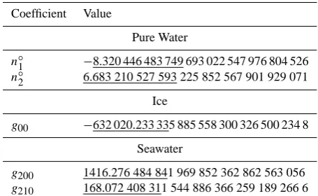
Table 1. The precise values of the adjustable coefficients of IAPWS-95 (pure fluid water), IAPWS-06 (pure ice) and IAPWS-08 (saline component of seawater) obtained from quadruple-precision code implementations. These coefficients were determined by en-suring the equality of the chemical potentials of liquid water, wa-ter vapor and of ice at the triple point, as well as the conditions Eq. (4a, b) for the saline part, as discussed in the section ”Refer-ence States”. The underlining in this table represents the accuracy with which these arbitrary adjustable constants can be determined by this procedure using double-precision code. In this paper when double-precision code (as opposed to quadruple-precision code) has been used to evaluate the thermodynamic properties of water ice and seawater, the arbitrary constants of this table have not been recomputed but rather the quadruple-precision determined values have been rounded to 15 significant figures and then used in the double-precision code. Note that this procedure gives more accurate values of some of these adjustable constants than can be obtained by evaluating them in double precision.
Coefficient Value
Pure Water
n◦1 −8.320 446 483 749 693 022 547 976 804 526 n◦2 6.683 210 527 593 225 852 567 901 929 071
Ice
g00 −632 020.233 335 885 558 300 326 500 234 8
Seawater
g200 1416.276 484 841 969 852 362 862 563 056 g210 168.072 408 311 544 886 366 259 189 266 6
the Lahey/Fujitsu Fortran 95 compiler1were used to promote all 64-bit real variables to 128-bit real variables and conver-gence tolerances were reduced until no change was observed to the desired number of digits. The quadruple-precision val-ues of coefficientsn◦1andn◦2determined from the Wagner-and-Pruß code (Table 1) were used.
Properties at the IAPWS-95 triple point, determined using the quadruple-precision codes described above, are given in Table 2 to the number of digits to which the two implemen-tations agree.
The properties of the numerical IAPWS-95/06 triple point have also been computed from a quadruple-precision imple-mentation of IAPWS-95 and IAPWS-06, as discussed below. If (T,p)is a good initial approximation to the numerical IAPWS-95/06 triple point (e.g.,T=273.16 K,p=611.655 Pa as reported by Wagner and Pruß, 2002), an iterative improve-ment can be obtained from the linearized equations
gIh−sIh1T +vIh1p=gW−sW1T +vW1p (1a)
Table 2. Numerical results for properties at the IAPWS-95 triple point obtained from quadruple-precision implementations. Here, g is the specific Gibbs energy andρ the density of liquid water (superscript W) and vapor (Vap). The underlined numbers indicate the digits that, based on our tests, can reasonably be expected to be reproduced using double-precision code.
Property Value Unit
T 273.16 K
pW 611.654 771 007 894 426 444 259 8×10⁻⁶ MPa pVap 611.654 771 007 894 426 444 259 8×10⁻⁶ MPa gW 0.611 781 703 456 382 623 667 3 J kg−1 gVap 0.611 781 703 456 382 623 667 3 J kg−1 ρW 999.792 520 031 620 646 603 898 354 735 kg m−3 ρVap 4.854 575 724 778 588 417 176 210×10−3 kg m−3
gIh−sIh1T +vIh1p=gVap−sVap1T +vVap1p , (1b) which have the solution
1T= g Ih−gW
vVap−vIh
− gIh−gVap
vW−vIh
sIh−sW
vVap−vIh−
sIh−sVap
vW−vIh (2a)
1p= s Ih−sW
gIh−gVap− sIh−sVap gIh−gW sIh−sW
vVap−vIh
− sIh−sVap
vW−vIh. (2b)
Here,gis the specific Gibbs energy, s the specific entropy andvthe specific volume of ice (superscript Ih), liquid wa-ter (W) and vapor (Vap). Use of this iwa-terative approach to determine successive improvements allows one to determine the numerical triple-point temperature and pressure values corresponding to the parameter values listed in the Releases. When this is done using quadruple-precision calculations, we find that Tt=273.160 000 093 070 855 667 516 123 4 K and pt=611.654 775 144 545 131 192 098 52×10−6MPa.
The deviation (almost 0.1µK) of the above estimate of the triple-point temperature from 273.16 K shows that a small modification of the adjustable coefficientg00 of the ice for-mulation IAPWS-06 is required for consistency with the ITS-90 temperature scale at this level of precision. Start-ing again withT=273.16 K, and using Eq. (1a, b) to itera-tively adjust1pandgIhwith1T=0, we find that the value
g00=−0.632 020 233 449 497×106published for the Gibbs function of ice (Feistel and Wagner, 2006; IAPWS, 2006), must be adjusted tog00=−0.632 020 233 335 886×106 to
correct the numerical IAPWS-95/06 triple-point temperature from the value given above toT=273.160 000 000 000 K in all 15 digits. This new value forg00 is expected to be
in-cluded in a future revised version of IAPWS-06. The more precise quadruple-precision estimate of g00 is given in
Ta-ble 1.
Determination of g00 completes the consistent determi-nation of all coefficients involved in the potential functions for pure water. The triple-point properties of all three wa-ter phases were computed in quadruple precision afwa-ter ad-justment of the coefficientsn◦1,n◦2andg00, and are reported
in Table 3. These results are given to the full precision for which stable results between iterations are obtained on one particular platform. Slight differences may occur on other platforms. Note that we use the full quadruple-precision co-efficients in Table 3 and in all of the tables presented in the appendix. The values presented are thus our best estimates of the true solutions, but will not be precisely reproduced by double-precision implementations. Underlining has thus been used in the tables given in this paper to indicate the dig-its that are expected to be reproduced by double-precision implementations. A discussion of the methods used to esti-mate what precision is achievable with double-precision im-plementations is given in the appendix.
It remains to allow for the influence of sea salt in seawater. In the seawater formulation (Feistel, 2008; IAPWS, 2008), the Gibbs function,g, of seawater is expressed as a sum of a water part,gW, derived from the IAPWS-95 Helmholtz po-tential, and a saline part,gS, as,
g(SA, T , p)=gW(T , p)+gS(SA, T , p) (3a) The functiongW(T,p)is related to the Helmholtz poten-tialfW(T,ρW)by the relation
gW(T , p)=fW(T , ρW)+ρW(T , p)×fρW(T , ρW) (3b) where the subscriptρonfWindicates partial differentiation withT constant and
ρW(T , p)=ρ(SA=0, T , p) (3c)
The salinity argument of the Gibbs function in Eq. (3) is the Absolute SalinitySA, which is the mass of dissolved mate-rial in seawater per unit mass of solution. For seawater of Reference Composition, Absolute Salinity is the same as the Reference-Composition Salinity (Millero et al., 2008).
It is convenient to adjust the free parameters determin-ing the reference levels of absolute energy and absolute en-tropy of sea salt such that enen-tropy and enthalpy of seawa-ter vanish for the standard ocean state (pSO=101 325 Pa, TSO=273.15 K, SSO=35.165 04 g kg−1). The related
ad-justable coefficients of the Gibbs function of seawater are
g200 and g210, i.e., its pressure-independent terms
propor-tional to salinity and to the powers 0 and 1 in temperature (Fofonoff, 1962; Feistel, 2003; IAPWS, 2008).
At its meeting in Warnem¨unde, Germany, in May 2006, WG127 chose to specify the arbitrary constants correspond-ing to the saline specific entropy,sS, and the saline specific enthalpy,hS, at the standard ocean state as
sS(SSO, TSO, pSO)=sW(Tt, pt)−sW(TSO, pSO) (4a)
Table 3. Quadruple-precision results for the properties of water, vapor and ice at the quadruple-precision estimate of the IAPWS-95 triple point given in Table 2 (T=273.16 K,p=611.654 771 007 894 426 444 259 8×10⁻⁶MPa), computed with the coefficients given in Table 1 of this paper. The underlined numbers indicate the digits that, based on our tests, can reasonably be expected to be reproduced using double-precision code.
Property Property of water Property of vapor Property of ice Unit
g 6.1178170345638262367E–1 6.1178170345638262367E–1 6.1178170345638262367E–1 J kg−1 (∂g/∂T )p –2.E–27a, 5.E–11a –9.1554934092985614572E+3 1.2206943393964807369E+3 J kg−1K−1
(∂g/∂p)T 1.0002075230252500703E–3 2.0599122491710824907E+2 1.0908581273666870118E–3 m3kg−1
(∂2g/∂T2)p –1.5448497277676153768E+1 –6.8983454098615831310 –7.6760298587519086996 J kg−1K−2
(∂2g/∂T ∂p) –6.7979215180919329145E–8 7.5819292780093068933E–1 1.7438796470007613398E–7 m3kg−1K−1
(∂2g/∂p2)T –5.0906231711021898838E–13 –3.3699243312745608812E–1 –1.2849594157169302559E–13 m3kg−1Pa−1 h 6.1178170345638262367E–1 2.5009151914656985040E+6 –3.3344425396783922172E+5 J kg−1 f 4.E–26a, 5.E–9a –1.2599490372460606626E+5 –5.5446874640188852815E–2 J kg−1 u 7.E–25a, 2.E–9a 2.3749196759593889814E+6 –3.3344492119641731829E+5 J kg−1 s 2.E–27a, –5.E–11a 9.1554934092985614572E+3 –1.2206943393964807369E+3 J kg−1K−1 ρ 9.9979252003162064660E+2 4.8545757247785884172E–3 9.1670949219948795011E+2 kg m−3 cp 4.2199115163700181633E+3 1.8843520321577900481E+3 2.0967843162166713804E+3 J kg−1K−1
α –6.7965110855503138742E–5 3.6807049820012030606E–3 1.5986310256590902275E–4 K−1 κT 5.0895669687676183977E–10 1.6359552852946201284E–3 1.1779344934788178705E–10 Pa−1
κs 5.0865762475261953085E–10 1.2314112503314651356E–3 1.1416159777876331107E–10 Pa−1
aEach of these numbers is identically zero in the theoretical model. The numbers shown here give the roundoff errors corresponding to quadruple- and double-precision implementations, respectively.
NOTE: The notationyE±nshould be interpreted asy×10±n.
Here,uW, hW andsW are the specific internal energy, en-thalpy and entropy of liquid water of the IAPWS-95 for-mulation, respectively, and (Tt, pt)refers to the numerical IAPWS-95 triple point as in Table 2. IAPWS-95 specifies the reference state conditionssW(Tt, pt)=0 and uW(Tt, pt)=0. The values ofg200andg210determined by Eq. (4) are given in Table 1 and numerical values of the quantities referred to in these equations are reported in additional tables in the ap-pendix.
The definitions Eq. (4a, b) have the following properties: 1. the free constants of the saline Gibbs energy, gS, are
specified, rather than those of the complete Gibbs en-ergy,g, of seawater,
2. the reference state definitions Eq. (4a, b) impose no con-ditions on the IAPWS-95 formulation,
3. the definitions Eq. (4a, b) require no additional explicit numerical values to be given,
4. the right sides of Eq. (4a, b) are independent of the choice of the two free constants within IAPWS-95, and so are the saline quantitiessS(SSO,TSO,pSO)and hS(SSO,TSO,pSO). In other words, the IAPWS
refer-ence state definition imposes no conditions on the for-mulation,gS(S,T,p),
5. the definitions are different from those given in Feis-tel (2003) only by the tiny misfit ofg(0,TSO,pSO)from
Feistel (2003) togW(TSO,pSO)from IAPWS-95, thus being comfortably consistent for oceanographers, and 6. the numerical absolute values ofs(SSO,TSO,pSO)and
h(SSO,TSO,pSO)for seawater depend on the
IAPWS-95 reference state in the same way as dosW(Tt,pt)and uW(Tt,pt)from IAPWS-95.
The properties of liquid water, ice and seawater at the stan-dard ocean state were computed in quadruple precision and are reported to 20 significant figures in Table A8 of the ap-pendix.
programming language, and on the way this code is executed by compilers or interpreters. There can of course be differ-ent implemdiffer-entations of the same mathematical model. They are all only approximations of the precise mathematical mod-els that they represent, but their numerical errors should be negligibly small compared to the uncertainties of the experi-mental data.
Things become more complicated when more than one formulation is considered and mutual consistency is required, as in the case of fluid water, ice and seawater. Although the mathematical models may be formulated to be exactly con-sistent, if the reference-point properties of ice are determined from an arbitrary implementation of fluid water properties and used as part of the mathematical model, then the theoret-ical formulation for ice becomes implementation-dependent rather than mathematically exact. If further formulations are integrated this way into a family of formulations, this proce-dure may eventually lead to significant inconsistencies within that family. Whether or not these inconsistencies are signif-icant will depend on the accuracy used to determine all pa-rameters that are determined based on consistency require-ments.
To consider a simple illustration, we imagine the follow-ing situation. The Gibbs function g(T, p) of liquid water is given (e.g., computed from IAPWS-95). To obtain a fast implementation, we develop separate correlation equations (i.e., mathematical models in our terminology) for each of its partial derivativesg,gT,gp,gT T,gT pandgpp. We only
re-quire that these correlation equations agree with the original formulation within the experimental uncertainty of entropy, density, etc. Using this approach, we will very probably ar-rive at a situation where our simplified separate equations in their combination no longer reproduce, say, the sound speed of the original formulation within its uncertainty.
The conclusion from these considerations is that the con-sistency between different but related formulations should al-ways be as precise as possible, in the ideal case mathemati-cally exact. If this consistency can be specified only numeri-cally, then the required relations should be computed with the highest achievable accuracy rather than within experimen-tal uncertainty only. In particular, the fundamenexperimen-tal mutual anchor points that impose consistency between the formula-tions should be very precisely determined in order to avoid unpredictable consequences for quantities derived from arbi-trary combinations of those formulations.
There are two different methods whereby this require-ment for rigorous consistency can be realized: the static and the dynamic definition of the adjustable coefficients. In the static method, the coefficients are computed based on the reference-state conditions with a high precision in advance, and the result of this computation is given as an explicit nu-merical value for each coefficient. The advantage of this method is that all implementations will use an identical set of coefficients, and the algorithms for fluid water, ice, and
the saline part of seawater can be implemented as modules independent of each other.
In the dynamic method, the adjustable coefficients are defined by the reference-state conditions in the form of equations rather than their solutions. These equations will be solved numerically during the run-time initializa-tion of each particular implementainitializa-tion, leading to slightly implementation-dependent values of the adjustable coeffi-cients which most accurately obey the conditions on the given platform.
For the quadruple-precision implementation used to com-pute the tables in the appendix, we have necessarily ap-plied the dynamic method. However, given that the re-sulting coefficients are very accurately determined and have been carefully verified, we recommend that the static values with 15 significant figures, obtained by rounding the coeffi-cients given in Table 1, be used in future work with double-precision code. This is already the recommendation for the Releases IAPWS-06 and IAPWS-08. We recommend that this approach also be taken for IAPWS-95 with coefficients determined from Table 1. This approach will be taken in the forthcoming source-code library (Feistel et al., 2009; Wright et al., 2009; McDougall et al., 2009b), where we will take all coefficients to be consistent with Table 1; this consistent set of coefficients is expected to be adopted by IAPWS in 2009 as minor revisions to the IAPWS-95 and IAPWS-06 releases. This approach provides the most accurate coefficients cur-rently available, the best possible consistency at the reference states obtainable with static values of all coefficients, and it will ensure that any inconsistencies between the results from different implementations are due to the details of the imple-mentation or the platform used to do the calculations, and not due to differences in the specification of coefficients. Tests reveal that differences between results on different platforms obtained using static coefficients should be entirely negligi-ble from a practical point of view.
Finally, we note that the mutually consistent family of for-mulations for water, ice and seawater will likely grow further in the future. Possible candidates are descriptions of aqueous sodium chloride solutions, of solid sea salt components and their saturation and precipitation from seawater, properties of humid air or gases dissolved in water, and the surface ten-sion and refractive index of seawater. There will certainly be a demand to consistently link such formulations to the exist-ing family. This will require highly accurate reference-state properties to be used for the determination of the coefficients of the added formulations. For this purpose, we provide in this paper tables of highly accurate reference values.
As an example of a potential need for such accuracy, one may at some future time wish to consider components of sea salt such as NaCl or CO2 in order to describe their
the Reference-Composition model (Millero et al., 2008). For components that contribute only, say, a fraction of 0.01% to the total mass of sea salt, their absolute internal energy may be defined with precision reduced by the same fraction. If the total internal energy of sea salt is available now with 15 cor-rect digits, only 11 accurate digits will be available for such a component, since all fractions need to sum up to give exactly 1. Thus, providing 19 digits for sea salt will permit a consis-tent specification of those components with 15 valid digits. For the same reason, the Reference Composition of sea salt itself was defined with more valid digits than required by the experimental uncertainties of its measurements, for example, to guarantee mathematically exact electrical neutrality of the resulting electrolyte model.
4 Metastable liquid water
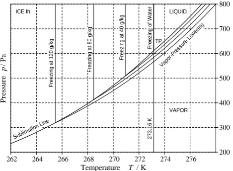
When sea salt is dissolved in water, the triple point defined by the equilibrium between seawater, ice and vapor is dis-placed from its pure-water locus along the sublimation line of pure water to lower pressures and temperatures (Fig. 4). As a consequence, stable liquid seawater is found at temper-atures and pressures where pure water is a metastable liquid, either subcooled or superheated. Thus, to determine seawater properties as a sum of pure water plus saline contributions, the properties of water in the metastable regimes are needed. A rough estimate of the amount by which the vapor pres-sure and the freezing temperature are lowered due to dis-solved sea salt can be determined from the thermodynamic equilibrium conditions in the form of the first terms of the related series expansions with respect to salinity, commonly known as Raoult’s laws.
The equilibrium between ice and seawater requires equal temperatures, pressures and chemical potentials of the water component in both phases, i.e.,
gIh=gW+gS−SA ∂gS ∂SA
!
T ,p
. (5a)
For a small depression value,1T/T, expanding Eq. (5a) in a power series in1T andS, we obtain approximately
1T T ≈ −
RST
hW−hIh ×SA ≈ −0.22×SA. (5b)
Here, RS=R/MS=264.7599 J kg−1K−1 is the specific gas
constant of sea salt, R is the molar gas constant,
MS=31.403 82 g mol−1is the molar mass of sea salt (Millero et al., 2008), and hW−hIh≈333 kJ kg−1 is the melting en-thalpy of ice. Adopted from the theory of ideal solutions (Feistel, 2008), the logarithmic term of the salinity expan-sion ofgSis responsible for Eq. (5b).
Similarly, the equilibrium condition between vapor and seawater,
262 264 266 268 270 272 274 276 200
300 400 500 600 700 800 P re ss u re p / P a
Temperature T / K
TP LIQUID
VAPOR ICE Ih
Sublim ation L
ine 2 7 3 .1 6 K F re e z in g o f W a te r F re e z in g a t 4 0 g /k g F re e z in g a t 8 0 g /k g F re e z in g a t 1 2 0 g /k g Vapo r-Pre ssur
e Lo
wer
ing
Fig. 4. Lowering of vapor pressure and of freezing temperature of seawater as a function of salinity in the vicinity of the pure-water triple point (TP). The four curves correspond to the four values of absolute salinity for which freezing temperatures are indicated on the diagram, with higher salinity values resulting in lowering of the vapor pressure for a given temperature. For non-zero salinities, the stable seawater phase occurs at temperature and salinity values for which the pure-water liquid phase is metastable. This figure is a magnified projection of Fig. 3 along the salinity axis. The projected triple line coincides with the sublimation line.
gVap=gW+gS−SA ∂g S
∂SA
!
T ,p
, (6a)
gives the analogous approximation for the vapor pressure lowering, as
1p p ≈ −
MW MS
×SA≈ −0.57×SA. (6b) Here, MW=18.015 268 g mol−1 is the molar mass of water (IAPWS 2001).
It is evident that for our purposes the mathematical func-tion gW(T, p) in Eq. (3) must produce reasonable values over the entire range of validity ofgS(SA,T,p). Some docu-mentation of reasonable metastable behaviour of IAPWS-95 was provided by Wagner and Pruß (2002), but an IAPWS task group was formed to investigate this issue more thor-oughly and concluded in its report given at the 2007 meeting in Lucerne that:
(i) the investigations established conclusively that IAPWS-95 behaves reasonably in the subcooled liquid range down to temperatures as low as 240 K;
(ii) IAPWS-95 functions are visually and numerically smooth in the subcooled region even at high pressures; (iii) an extensive literature search made in 2005 did not
(iv) IAPWS-95 is in satisfactory agreement with existing ex-perimental data for subcooled water (density, heat ca-pacity, speed of sound) at normal pressure;
(v) there are no data for subcooled water at high pressures (the values discussed in some papers are computed ex-clusively from models or extrapolation); and
(vi) there is no better option than IAPWS-95 as the pure wa-ter reference for the seawawa-ter formulation.
Regarding point (v), recent density measurements below 0◦C at high pressures (Sotani et al., 2000; Asada et al., 2002) agree with IAPWS-95 within 0.05% over the oceanographic pressure range up to 100 MPa.
As is evident from Fig. 4, the metastable liquid range re-quired for use in the determination of seawater properties us-ing the form Eq. (3) extends to pressures and temperatures that are well below those corresponding to the triple point of pure water. For seawater applications, code implement-ing IAPWS-95 should allow consideration of the full range of property values indicated in Fig. 4, rather than being re-stricted to the region of the stable liquid phase. (Such an application of IAPWS-95 corresponds to an extrapolation of this formulation.) A new version of the code that allows con-sideration of the full range of seawater conditions of interest will be made available in Feistel et al. (2009) and Wright et al. (2009).
5 Discussion
The SCOR/IAPSO Working Group 127 (WG127) was formed in 2005 and charged with developing a new seawa-ter standard for oceanography to replace the Inseawa-ternational Equation of State of Seawater (EOS-80, Fofonoff and Mil-lard 1983) that has served the needs of oceanographers for nearly three decades. The general approach taken by WG127 has been to develop a Gibbs function formulation that can be applied over the full range of conditions of interest including pure water, seawater and sea ice.
The IAPWS-95 Helmholtz potential function (Wagner and Pruß, 2002) has served as the starting point from which the Gibbs function for pure water has been determined. This was complemented by Feistel and Wagner (2006) by the intro-duction of a Gibbs potential for salt-free ice, thus completing the required set of Gibbs functions for pure water, including solid, liquid and vapor phases.
The solid-liquid-gas triple point plays a special role in Gibbs function (and other) formulations of the thermody-namic properties of seawater. In particular, it serves as a reference point at which entropy and internal energy of the liquid water phase are commonly set to zero to determine two free parameters in the formulation. Once these two free parameters for the liquid phase are set, an additional free pa-rameter that enters the formulation of the Gibbs potential for
the solid phase must be chosen consistent with the definition of the ITS-90 temperature scale for which the value 273.16 K is defined by the triple point. A consequence of this fact is that any change in the Gibbs function for pure water that re-sults in a change in the value of the Gibbs potential for liquid and vapor at the triple point will require an adjustment of the free parameter in the Gibbs function for the solid phase in order to retain the property that the temperature is exactly 273.16 K at this point.
Unfortunately, the numerical implementation of the code used by Feistel and Wagner (2006) had its parameters rounded off to slightly lower precision than those listed in the IAPWS-95 release, thus resulting in a very small but non-zero deviation from the strict IAPWS-95 definition of the Helmholtz function. While this difference results in changes that are well within measurement uncertainties, the adjust-ment to achieve strict consistency with IAPWS-95 results in a small inconsistency between the physical definition of the triple point and the requirement that the temperature at the triple point be 273.16 K on the ITS-90 temperature scale. In Sect. 3, we have thus adjusted the free parameterg00to very
precisely satisfy this condition. To achieve highly accurate results (and much more accurate than required for consis-tency with observations), we have used quadruple-precision numerical code in this exercise, resulting in the adjusted valueg00=−0.632 020 233 335 886×106 when rounded to double precision.
With code in precise agreement with IAPWS-95 and prop-erly adjusted to the reference state conditions, and the correc-tion of the parameterg00as required to maintain consistency with the ITS-90 temperature scale, Table 1, the Gibbs func-tion formulafunc-tion for pure water is complete and fully consis-tent.
To complete the Gibbs function formulation for seawater, the Gibbs potential associated with salinity effects has been determined by Feistel (2008) and added to the Gibbs poten-tial for pure water as in Eq. (3). Use of this form for the Gibbs function of seawater ensures consistency with the Helmholtz formulation for pure water, but requires some special consid-erations for its application. In particular, to use Eq. (3) over the desired application range for seawater, it has been neces-sary to extend the range of application of the Gibbs function for pure water to temperature and pressure values for which seawater is a stable liquid, but the stable phase of pure water is ice Ih or vapor. Thus metastable states of liquid water have been examined, as discussed in Sect. 4.
Table A1. Quadruple-precision values corresponding to results published in Table 6 of IAPWS-95 with the coefficients given in Table 1 of this paper. The ideal-gas partφ◦and the residual partφrof the dimensionless Helmholtz free energy together with the corresponding derivativesa are shown forT=500 K and ρ=838.025 kg m−3. The underlined numbers indicate the digits that, based on our tests, can reasonably be expected to be reproduced using double-precision code.
φ◦ 2.047977334795977679296586756701 φr –3.426932056815592848942243599952 φδ◦ 0.3842367471137495898093732287223 φδr –0.3643666503638817298034879725024 φδδ◦ –0.1476378778325555537348148082081 φδδr 0.8560637009746113823633081128560 φτ◦ 9.046111061752422039021337148156 φτr –5.814034352384169258028794246361 φτ τ◦ –1.932491850130520326231797178581 φτ τr –2.234407368843363755796662019232
φδτ◦ 0 φδτr –1.121769146703061888902147087817
aFor the abbreviated notation of the derivatives ofφ◦
andφrsee the footnotes of Tables 4 and 5 of IAPWS-95, respectively.
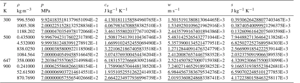
Table A2. Quadruple-precision results for water properties in the single-phase region at the selected values ofT andρpublished in Table 7 of IAPWS-95 with the coefficients given in Table 1 of this paper. The underlined numbers indicate the digits that, based on our tests, can reasonably be expected to be reproduced using double-precision code.
T ρ p cv w s
K kg m−3 MPa J kg−1K−1 m s−1 J kg−1K−1
300 996.5560 9.9241835181379651094E–2 4.1301811158584960765E+3 1.5015191380813064465E+3 0.39306264288077403467E+3 1005.308 2.0002251528132528836E+1 4.0679834708858382510E+3 1.5349250109621962916E+3 0.38740540099921296375E+3 1188.202 7.0000470354978172066E+2 3.4613558020377671029E+3 2.4435799167401894386E+3 0.13260961642075693598E+3 500 0.435000 9.9967942317602231789E–2 1.5081754139110436746E+3 5.4831425265432771044E+2 7.9448827136464213826E+3
4.532000 9.9993812483991278912E–1 1.6699102452455069490E+3 5.3573900134521477951E+2 6.8250272527689584303E+3 838.0250 1.0000385800922118506E+1 3.2210621867405833518E+3 1.2712844091476324779E+3 2.5669091854222539144E+3 1084.564 7.0000040549458516645E+2 3.0743769300454436204E+3 2.4120087657446758352E+3 2.0323750919066389535E+3 647 358.0000 2.2038475570652149984E+1 6.1831572766683092166E+3 2.5214507827000715938E+2 4.3209230667550033099E+3 900 0.241000 1.0006255868266188154E–1 1.7589065704448138520E+3 7.2402714652918938252E+2 9.1665319385523842681E+3 52.61500 2.0000069037214614551E+1 1.9351052551262241493E+3 6.9844567383679534276E+2 6.5907022485101277853E+3 870.7690 7.0000000575565402666E+2 2.6642234977936996739E+3 2.0193360824868338741E+3 4.1722380158463258117E+3
of the PSS-78 salinity scale. Of couse, other limitations re-main. For example, depending on the temperature, the su-persaturation of high-salinity seawater may cause the precip-itation of calcium minerals and thus a composition change of dissolved sea salt (Marion et al., 2008a, b). Composition anomalies due to this or other effects will degrade the accu-racy of Reference-Composition Salinity as a measure of the Absolute Salinity used in the Gibbs function formulation of Feistel (2008). Such anomalies need to be taken into account to minimize inaccuracies.
The combination of the Helmholtz function for pure wa-ter, the Gibbs potential for salt-free ice and the saline part of the Gibbs potential for seawater provides a unified and fully consistent foundation for the consideration of the thermody-namic properties of pure water and seawater.
Mathematically, the combination of a Helmholtz func-tion for the pure-water part with a Gibbs funcfunc-tion for the saline part requires a proper use of theoretical thermody-namic methods and is not always a trivial exercise. For con-venience of application, WG127 is implementing the new set of thermodynamic functions for liquid water, water vapor, ice, and seawater, as well as their mutual phase equilibria,
in a comprehensive source code library for oceanographers and other scientists and engineers who deal with seawater (Feistel et al., 2009; Wright et al., 2009; McDougall et al., 2009b). In addition to the precise implementations of the relations discussed herein, efficient and accurate approxima-tions for some quantities that require computationally effi-cient implementations will also be provided. Quantities such as entropy and enthalpy of seawater, which were not avail-able from EOS-80, result naturally from the Gibbs function formalism, and the WG127 source code will include these quantities.
Appendix A
Table A3. Quadruple-precision results for property values in the two-phase region at the selected values of temperature published in Table 8 of IAPWS-95 with the coefficients given in Table 1 of this papera. The underlined numbers indicate the digits that, based on our tests, can reasonably be expected to be reproduced using double-precision code.
Property T=275 K T=450 K T=625 K Unit
pW 6.9845116670084935279E–4 9.3220356362820145516E–1 1.6908269318578409807E+1 MPa pVap 6.9845116670084935279E–4 9.3220356362820145516E–1 1.6908269318578409807E+1 MPa ρW 9.9988740611984984069E+2 8.9034124976167258553E+2 5.6709038514635254862E+2 kg m−3 ρVap 5.5066491850412278079E–3 4.8120036012567123262 1.1829028045115688596E+2 kg m−3 hW 7.7597220155398177939E+3 7.4916158501216908622E+5 1.6862697594697419575E+6 J kg−1 hVap 2.5042899500405145942E+6 2.7744107798896210429E+6 2.5507162456234704801E+6 J kg−1 sW 2.8309466959519726149E+1 2.1086584468844730194E+3 3.8019468301114322634E+3 J kg−1K−1 sVap 9.1066012052321552768E+3 6.6092122132788107010E+3 5.1850612079573978994E+3 J kg−1K−1
aEach of these test values was calculated from the Helmholtz free energy by applying the phase-equilibrium condition (Maxwell criterion).
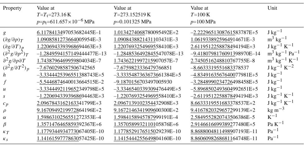
Table A4. Quadruple-precision results for the properties of pure ice at the triple point, the normal-pressure melting point and atT=100 K, p=100 MPa. Results correspond to Table 6 of IAPWS-06 with the corrected coefficientg00of ice given in Table 1. The underlined numbers indicate the digits that, based on our tests, can reasonably be expected to be reproduced using double-precision code.
Property Value at Value at Value at Unit
T=Tt=273.16 K T=273.152519 K T=100 K
p=pt=611.657×10⁻⁶MPa p=0.101325 MPa p=100 MPa
g 6.1178413497053682445E–1 1.0134274068780095492E+2 –2.2229651308761583787E+5 J kg−1 (∂g/∂p)T 1.0908581273664005954E–3 1.0908438821431103431E–3 1.0619338925964914671E–3 m3kg−1
(∂g/∂T )p 1.2206943393968694463E+3 1.2207693254969558410E+3 2.6119512258878494194E+3 J kg−1K−1
(∂2g/∂p2)T –1.2849594157149444477E–13 –1.2848536492845547078E–13 –9.4180798176091398970E–14 m3kg−1Pa−1
∂2g/∂p∂T 1.7438796469959804034E–7 1.7436221997215907057E–7 2.7450516248810767755E–8 m3kg−1K−1
(∂2g/∂T2)p –7.6760298587506742565 –7.6759823336479766851 –8.6633319551683378537 J kg−1K−2
h –3.3344425396551388743E+5 –3.3335487363673661384E+5 –4.8349163567640077981E+5 J kg−1 f –5.5446874640013664515E–2 –9.1870156703497005930 –3.2848990234726498458E+5 J kg−1 u –3.3344492119652349798E+5 –3.3346540339309476449E+5 –5.8968502493604992651E+5 J kg−1 s –1.2206943393968694463E+3 –1.2207693254969558410E+3 –2.6119512258878494194E+3 J kg−1K−1 cp 2.0967843162163341799E+3 2.0967139102354432908E+3 8.6633319551683378537E+2 J kg−1K−1
ρ 9.1670949219972864196E+2 9.1672146341909600300E+2 9.4167820329657299139E+2 kg m−3 α 1.5986310256551272353E–4 1.5984158945787999191E–4 2.5849552820743506386E–5 K−1 β 1.3571476465859392367E+6 1.3570589932110105876E+6 2.9146616699389277480E+5 Pa K−1 κT 1.1779344934773067405E–10 1.1778529176515029239E–10 8.8688004811498907193E–11 Pa−1 κs 1.1416159777863057425E–10 1.1415444255649804160E–10 8.8606098268681164748E–11 Pa−1
numbers with more digits than required by the experimental accuracy. They report fewer digits than available from a typ-ical 64-bit floating point number and suppress the part which very likely varies between different implementations, since those digits may be more confusing than helpful for the ex-amination of the code’s correctness. Thus, with respect to these published check values, all correct and well-organised implementations are considered equally good.
For certain applications of the Releases, as e.g. for the development of a source code library for seawater, it is im-portant to estimate the implementation errors, i.e., the devia-tions from the mathematical formuladevia-tions. This is of interest
when speed-optimized code is required for circulation mod-els or other time-critical applications, to monitor the degree to which the precision of the results is diminished by certain accelerating modifications or simplifications. This is also of interest to see the effects of reorganising internal details of the code, the sequence of execution, the grouping into proce-dures, etc.
Table A5. Quadruple-precision results for the water part, saline part and total properties published in Table 8a of IAPWS-08 with the coef-ficients given in Table 1 of this paper. Properties atSA=Sn=0.035 165 04 kg kg−1,T=T0=273.15 K,p=p0=0.101325 MPa. The underlined numbers indicate the digits that, based on our tests, can reasonably be expected to be reproduced using double-precision code.
Property Water part Saline part Property of seawater Unit
g 1.0134274172939062882E+2 –1.0134274172939062882E+2 –2.E–29b, 4.E–9b J kg−1 (∂g/∂SA)T ,p 0.0 6.3997406731229904527E+4 6.3997406731229904527E+4 J kg−1
(∂g/∂T )S,p 1.4764337634625266531E–1 –1.4764337634625266531E–1 7.E–32b, –6.E–11b J kg−1K−1
(∂g/∂p)S,T 1.0001569391216926347E–3 –2.7495722426843287457E–5 9.7266121669484934729E–4 m3kg−1
(∂2g/∂SA∂p)T 0.0 –7.5961541151530889445E–4 –7.5961541151530889445E–4 m3kg−1
(∂2g/∂T2)S,p –1.5447354231977289339E+1 8.5286115117592251026E–1 –1.4594493080801366829E+1 J kg−1K−2 (∂2g/∂T ∂p)S –6.7770031786558265755E–8 1.1928678741395764132E–7 5.1516755627399375563E–8 m3kg−1K−1
(∂2g/∂p2)S,T –5.0892889464349017238E–13 5.8153517233288224927E–14 –4.5077537741020194745E–13 m3kg−1Pa−1
h 6.1013953480411713295E+1 –6.1013953480411713295E+1 –4.E–29b, 2.E–8b J kg−1 f 1.8398728851226087838E–3 –9.8556737654490732723E+1 –9.8554897781605610114E+1 J kg−1 u –4.0326948376093792920E+1 –5.8227949405511817194E+1 –9.8554897781605610114E+1 J kg−1 s –1.4764337634625266530E–1 1.4764337634625266531E–1 –7.E–32b, 6.E–11b J kg−1K−1
ρ 9.9984308550433049647E+2 –a 1.0281071999540078127E+3 kg m−3
cp 4.2194448084645965831E+3 –2.3295902344370323368E+2 3.9864857850208933494E+3 J kg−1K−1
w 1.4023825310882262606E+3 –a 1.4490024636214836206E+3 m s−1
µW 1.0134274172939062882E+2 –2.3518141093293594707E+3 –2.2504713675999688419E+3 J kg−1
aThe quantitiesρandware nonlinear ingand hence cannot be computed fromgSalone.
bEach of these numbers is identically zero in the theoretical model. The numbers shown here give the roundoff errors corresponding to quadruple- and double-precision implementations, respectively.
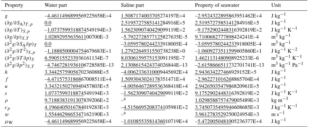
Table A6. Quadruple-precision results for the water part, saline part and total properties published in Table 8b of IAPWS-08 with the coefficients given in Table 1 of this paper. Properties atSA=0.1 kg kg−1=100 g kg−1,T=353 K,p=p0=0.101325 MPa. This point is located in the regions with restricted validity. The underlined numbers indicate the digits that, based on our tests, can reasonably be expected to be reproduced using double-precision code.
Property Water part Saline part Property of seawater Unit
g –4.4611496899569225658E+4 1.5087174003705274197E+4 –2.9524322895863951462E+4 J kg−1 (∂g/∂SA)T ,p 0.0 2.5195727585141284916E+5 2.5195727585141284916E+5 J kg−1
(∂g/∂T )S,p –1.0737599318874549194E+3 1.5623090740429099119E+2 –9.1752902448316392819E+2 J kg−1K−1 (∂g/∂p)S,T 1.0289295563561100700E–3 –5.7922728577125827635E–5 9.7100682777898424241E–4 m3kg−1
(∂2g/∂SA∂p)T 0.0 –3.0595780244233918005E–4 –3.0595780244233918005E–4 m3kg−1
(∂2g/∂T2)S,p –1.1888500004754679683E+1 1.2792264931550738238E+0 –1.0609273511599605860E+1 J kg−1K−2
(∂2g/∂T ∂p)S 6.5905155233936161134E–7 8.0306159575153091195E–7 1.4621131480908925233E–6 m3kg−1K−1
(∂2g/∂p2)S,T –4.7467281936106728585E–13 2.1308615424374026844E–13 –2.6158666511732701741E–13 m3kg−1Pa−1 h 3.3442575905670236088E+5 –4.0062336310009445692E+4 2.943634227466929152E+5 J kg−1 f –4.4715753186867008511E+4 1.5093043024178351471E+4 –2.962271016268865704E+4 J kg−1 u 3.3432150276940457803E+5 –4.0056467289536368418E+4 2.9426503547986820961E+5 J kg−1 s 1.0737599318874549194E+3 –1.5623090740429099119E+2 9.1752902448316392819E+2 J kg−1K−1
ρ 9.7188383191307839206E+2 –a 1.0298588757479005489E+3 kg m−3
cp 4.1966405016784019283E+3 –4.5156695208374105981E+2 3.7450735495946608685E+3 J kg−1K−1
w 1.5544629665347162190E+3 –a 3.9612783529250024954E+3 m s−1
µW –4.4611496899569225658E+4 –1.0108553581436010719E+4 –5.4720050481005236377E+4 J kg−1
Table A7. Quadruple-precision results for the water part, saline part and total properties published in Table 8c of IAPWS-08 with the coefficients given in Table 1 of this paper. Properties atSA=0.035 165 04 kg kg−1,T=T0=273.15 K,p=100 MPa. The underlined numbers indicate the digits that, based on our tests, can reasonably be expected to be reproduced using double-precision code.
Property Water part Saline part Property of seawater Unit
g 9.7730386219537338734E+4 –2.6009305073063660852E+3 9.5129455712230972649E+4 J kg−1 (∂g/∂SA)T ,p 0.0 –5.4586158064879659787E+3 –5.4586158064879659787E+3 J kg−1
(∂g/∂T )S,p 8.5146650206262343669E+0 7.5404568488116539426E+0 1.6055121869437888309E+1 J kg−1K−1
(∂g/∂p)S,T 9.5668332915350911569E–4 –2.2912384179113101721E–5 9.3377094497439601397E–4 m3kg−1
(∂2g/∂SA∂p)T 0.0 –6.4075761854574757172E–4 –6.4075761854574757172E–4 m3kg−1
(∂2g/∂T2)S,p –1.4296987338759055994E+1 4.8807697394225122581E–1 –1.3808910364816804768E+1 J kg−1K−2
(∂2g/∂T ∂p)S 1.9907957080315389517E–7 4.6628441224121312517E–8 2.4570801202727520769E–7 m3kg−1K−1
(∂2g/∂p2)S,T –3.7153088942341756981E–13 3.5734573584532666554E–14 –3.3579631583888490325E–13 m3kg−1Pa−1
h 9.5404605469153282817E+4 –4.6606062955592693597E+3 9.0743999173594013457E+4 J kg−1 f 2.0620533041864271652E+3 –3.0969208939505591314E+2 1.7523612147913712521E+3 J kg−1 u –2.6372744619762875211E+2 –2.3693678776479591876E+3 –2.6330953238455879397E+3 J kg−1 s –8.5146650206262343669E+0 –7.5404568488116539426E+0 –1.6055121869437888309E+1 J kg−1K−1
ρ 1.0452779613969214514E+3 –a 1.0709264465574263352E+3 kg m−3
cp 3.9052220915820361447E+3 –1.3331822543232592233E+2 3.7719038661497102223E+3 J kg−1K−1
w 1.5754223984859303496E+3 –a 1.6219899764987563752E+3 m s−1
µW 9.7730386219537338734E+4 –2.4089780641265845021E+3 9.5321408155410754232E+4 J kg−1
aThe quantitiesρandware nonlinear ingand hence cannot be computed fromgSalone.
Table A8. Quadruple-precision results for the properties of water, ice and seawater at the standard ocean state, computed with all coefficients as given in Table 1 of this paper.T=273.15 K,p=0.101 325 MPa andSA=0.035 165 04 for seawater. The underlined numbers indicate the digits that, based on our tests, can reasonably be expected to be reproduced using double-precision code.
Property Property of water Property of ice Property of seawater Unit
g 1.0134274172939062882E+2 9.8267598403431717064E+1 –2.E–29a, 4.E–9a J kg−1
(∂g/∂SA)T ,p 0.0 0.0 6.3997406731229904527E+4 J kg−1
(∂g/∂T )S,p 1.4764337634625266531E–1 1.2207886612999530642E+3 7.E–32a, –6.E–11a J kg−1K−1
(∂g/∂p)S,T 1.0001569391216926347E–3 1.0908434429264352467E–3 9.7266121669484934729E–4 m3kg−1
(∂2g/∂SA∂p)T 0.0 0.0 –7.5961541151530889445E–4 m3kg−1
(∂2g/∂T2)S,p –1.5447354231977289339E+1 –7.6759851115667509185E+0 –1.4594493080801366829E+1 J kg−1K−2
(∂2g/∂T ∂p)S –6.7770031786558265755E–8 1.7436082496084962410E–7 5.1516755627399375563E–8 m3kg−1K−1
(∂2g/∂p2)S,T –5.0892889464349017238E–13 –1.2848482463976179327E–13 –4.5077537741020194745E–13 m3kg−1Pa−1 h 6.1013953480411713295E+1 –3.3336015523567874778E+5 –4.E–29a, 2.E–8a J kg−1 f 1.8398728851226087838E–3 –1.2262113451089334305E+1 –9.8554897781605610114E+1 J kg−1 u –4.0326948376093792920E+1 –3.3347068494753326883E+5 –9.8554897781605610114E+1 J kg−1 s –1.4764337634625266531E–1 –1.2207886612999530642E+3 –7.E–32a, 6.E–11a J kg−1K−1 ρ 9.9984308550433049647E+2 9.1672183252738167257E+2 1.0281071999540078127E+3 kg m−3 cp 4.2194448084645965831E+3 2.0966953332244580134E+3 3.9864857850208933494E+3 J kg−1K−1 α –6.7759397686198971741E–5 1.5984037497909609918E–4 5.2964747378800447017E–5 K−1 κT 5.0884903632265555122E–10 1.1778484389572171289E–10 4.6344541107741383004E–10 Pa−1 κs 5.0855176492808069170E–10 1.1415405263722770087E–10 4.6325845206948706884E–10 Pa−1
µW 1.0134274172939062882E+2 9.8267598403431717064E+1 –2.2504713675999688419E+3 J kg−1
Table A9. Formulas for properties reported in Tables A2–A8, expressed in terms of partial derivatives of the Helmholtz functionf (T,ρ) of fluid water and the Gibbs functionsg(T,p)of ice andg(SA,T,p)of seawater.
Property Expression in Expression in Expression in Comment
g(S, T, p) of seawater g (T, p) of ice f (T,ρ) of fluid water
g g g f+ρfρ specific Gibbs energy
(∂g/∂SA)T ,p gS 0 0
(∂g/∂T )S,p gT gT fT
(∂g/∂p)S,T gp gp ρ−1
(∂2g/∂SA∂p)T gSp 0 0
(∂2g/∂T2)S,p gT T gT T fT T−ρfρT2 / 2fρ+ρfρρ
(∂2g/∂T ∂p)S gT p gT p fρT/
2ρfρ+ρ2fρρ
(∂2g/∂p2)S,T gpp gpp −1/
n
ρ3 2fρ+ρfρρ
o
h g−T gT g−T gT f−T fT+ρ fρ specific enthalpy
f g−p gp g−p gp f specific Helmholtz energy
u g−T gT−p gp g−T gT−p gp f−T fT specific internal energy
s –gT –gT –fT specific entropy
p p p ρ2fρ pressure
ρ 1/gp 1/gp ρ density
cp –T gT T –T gT T T
n
ρfT ρ2 2fρ+ρfρρ−fT T
o
specific isobaric heat capacity
α gT p/gp gT p/gp fT ρ/ 2fρ+ρfρρ thermal expansion
κT –gpp/gp –gpp/gp 1/
n
ρ2 2fρ+ρfρρ
o
isothermal compressibility
κs
gT p2 −gT T gpp
/ gpgT T
g2T p−gT Tgpp
/ gpgT T
fT T/nρ2fT T 2fρ+ρfρρ−ρ3fT ρ2
o
isentropic compressibility
w gp
r
gT T/
g2T p−gT Tgpp
–a
r
ρ2
fT Tfρρ−fρT2
/fT T+2ρfρ sound speed
µW g−SAgS g f+ρfρ chemical potential of water
β – –gT p/gpp – pressure coefficient for ice
aSound speeds in solid crystals cannot be computed from volume compressibility.
In addition to these tables with numerical check values, we report in this appendix properties of liquid water, water vapor, ice and seawater at the reference states explained in Sect. 3.
Underlining in all tables shows the digits of the more accu-rate quadruple-precision results that typical double-precision implementations of the fluid, ice and seawater potential func-tions should be able to reproduce. This underlining was de-termined using two independent techniques. The first method is based on a manual comparison of double- and quadruple-precision results and the observation that different implemen-tations of the potential functions in double-precision arith-metic give the same agreement with the quadruple-precision table entries to within one digit. We compared two differ-ent implemdiffer-entations in two differdiffer-ent languages on differdiffer-ent machines and operating systems. Both implementations used the values of the arbitrary adjustable constants as listed in Ta-ble 1 but rounded to 15 decimal digits, as is consistent with double-precision code.