www.atmos-meas-tech.net/7/1693/2014/ doi:10.5194/amt-7-1693-2014
© Author(s) 2014. CC Attribution 3.0 License.
Cloud shadow speed sensor
V. Fung, J. L. Bosch, S. W. Roberts, and J. Kleissl
Department of Mechanical and Aerospace Engineering, University of California, San Diego, California, USA Correspondence to: J. Kleissl ([email protected])
Received: 13 June 2013 – Published in Atmos. Meas. Tech. Discuss.: 22 October 2013 Revised: 18 March 2014 – Accepted: 23 April 2014 – Published: 12 June 2014
Abstract. Changing cloud cover is a major source of solar radiation variability and poses challenges for the integration of solar energy. A compact and economical system is pre-sented that measures cloud shadow motion vectors to esti-mate power plant ramp rates and provide short-term solar irradiance forecasts. The cloud shadow speed sensor (CSS) is constructed using an array of luminance sensors and a high-speed data acquisition system to resolve the progression of cloud passages across the sensor footprint. An embedded microcontroller acquires the sensor data and uses a cross-correlation algorithm to determine cloud shadow motion vec-tors. The CSS was validated against an artificial shading test apparatus, an alternative method of cloud motion detection from ground-measured irradiance (linear cloud edge, LCE), and a UC San Diego sky imager (USI). The CSS detected artificial shadow directions and speeds to within 15◦ and 6 % accuracy, respectively. The CSS detected (real) cloud shadow directions and speeds with average weighted root-mean-square difference of 22◦and 1.9 m s−1when compared to USI and 33◦and 1.5 m s−1when compared to LCE results.
1 Introduction
Given the impact of fossil fuel consumption on the environ-ment, it is imperative that renewable energy sources provide a greater fraction of world energy demand. On average, the Earth receives 8000 times more solar energy than the energy consumed globally, making solar energy a strong candidate for supplying future world energy needs. However, difficul-ties in integrating variable generators into the electric grid have impacted the rate of large-scale adoption of solar power. The variability of the solar resource could be better accom-modated by grid operators if fluctuations in irradiance caused by cloud cover could be predicted.
Understanding cloud motion is critical for ramp rate esti-mation and short-term forecasting (Arias-Castro et al., 2013; Coimbra et al., 2013; Lave et al., 2012, 2013), because cloud motion causes a sudden shortage or oversupply in solar power and must be compensated for with an opposing ramp of energy storage or conventional generation. Previous stud-ies have used satellite imagery for estimating cloud motion (Leese et al., 1971; Hammer et al., 1999; Lorenz et al., 2004; Perez et al., 2010). However, due to satellite navigation, res-olution, and parallax uncertainties, such cloud motion esti-mates are of limited use in very short-term, intra-hour fore-casting.
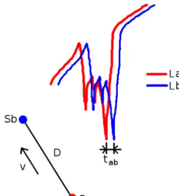
Figure 1. Idealized sketch showing the most correlated pair of
sig-nals shifted bytab(adapted from Bosch et al., 2013).
al. (2013) using ground-based solar radiation measurements. The first approach (further developed in Bosch and Kleissl, 2013) considers the kinematic equations of a linear cloud edge (LCE) passing through a sensor triplet and will be used in this paper for validation. The second method is based on the most correlated pair (MCP) of sensors arranged in 12 m diameter semi-circular array and lays the foundation of the cloud shadow speed sensor (CSS) described here. However, the limited sampling frequency requires sensor spacings of tens of meters and does not permit detecting cloud speeds with enough resolution to cover the full range of naturally oc-curring cloud speeds. Also, the system is not self-contained and cannot perform on-board post-processing. A semicircle system that is smaller, self-contained, and sampling at high frequency is required for commercial use, and is described in this paper.
Section 2 describes the theoretical concept for the cloud motion vector (CMV) measurement. Sections 3.1 and 3.2 desribes the phototransistor characteristics, optical assem-bly, and layout. In Sect. 3.3 the data acquisition and post-processing system is presented and quality control is dis-cussed. Performance parameters and limitations of the CSS are explained in Sect. 3.4. Validation procedures for the algo-rithm and cloud motion results against artificial shadows and (real) clouds are described in Sects. 3.5 and 3.6, and results of the validation are shown in Sect. 4.
2 Theory: most correlated pair method (MCP)
Variability of solar irradiance at the Earth’s surface is mainly due to cloud shadows with varying light intensity. We present here a system to obtain CMVs using an array of ground-based sensors to measure the spatiotemporal variation of
Figure 2. cloud shadow speed sensor (CSS). The entire system is
contained inside a weather-proof enclosure. On the top of the enclo-sure is an array of nine phototransistors used to meaenclo-sure the varia-tion in solar radiavaria-tion as clouds passed overhead.
solar irradiance over the extent of the sensor array. Using the MCP method described in Bosch et al. (2013), the largest similarity in a pair of signals indicates alignment with the direction of cloud motion and is determined by the cross-correlation coefficientRab(1t ):
Rab(1t )= (1)
1 n−1
Xn
m=1
La,t(m)− ¯La,t ˆ
La,t
!
Lb,t+1t(m)− ¯Lb,t+1t ˆ
Lb,t+1t
!
,
whereaandbare sensor indices,nis the number of sample points,tandt+1tare the time and lagged time,LaandLb are solar irradiance time series, overbars indicate averages, and hats indicate standard deviations.
Assuming sensorsSaandSbare the pair with largestRab, the detected solar irradiance time series will be most similar but delayed by a time lag,1t=tab, as seen in Fig. 1.
Determining the time lag via cross correlation, the cloud speed can be found by
Vcloud=
D tab
, (2)
whereDis the distance separating the sensors.
3 Cloud shadow speed sensor (CSS)
Figure 3. Simplified schematic showing excitation voltage applied
to the phototransistor collector, the 2kload resistor, and the
sen-sor output as applied to an analog input channel on the microcon-troller.
3.1 Luminance sensors
Solar radiation sensors consist of an array of nine phototran-sistors (TEPT4400, Vishay Intertechnology Inc., USA). The sensors have a spectral response ranging from approximately 350 to 1000 nm with a peak response at 570 nm. The manu-facturer has characterized the sensors over an operating tem-perature range of −40 to+85◦C. Response time was de-termined experimentally in our laboratory and found to be 21 µs rise time (10–90 % response). Excitation voltage for the sensors was 3.3 VDC supplied from a voltage regulator (LM2937-3.3, Texas Instruments Inc., USA) and applied to the phototransistor collector (Fig. 3). A 2k load resistor was connected from the sensor emitter to system ground. The sensor outputs were taken at the emitter–load-resistor junc-tion and fed to the analog input channels on the microcon-troller.
3.2 Luminance sensor array
CMVs were determined with the phototransistors configured as an array of eight sensors positioned around a central sen-sor on a circle of radius 0.297 m, covering 0–105◦in 15◦ in-crements (Figs. 2 and 4). Cross-correlation coefficients were computed for each pair of sensors (central sensor and a sen-sor on the circle) to determine cloud speed and direction based on Eqs. (1)–(2).
Each sensor was placed at the base of and inside a black opaque tube with a diameter of 6.35 mm and height of 14.3 mm with a translucent acrylic light diffuser/collector at the top. The tube height was chosen such that the diffuser positioned above the sensor fully occupies the TEPT4400 field of view (FOV) as shown in Fig. 5. Full exposure of the TEPT4400 sensor FOV to the overhead light field dic-tates a vertical separation ofh <5.51 mm, buth=2.78 mm was chosen in the design such that a tilt error of up to 18.8◦ would still allow the TEPT4400 FOV to remain within the diffuser area. This sensor optical assembly (TEPT4400, tube,
Figure 4. Sensor arrangement. Each circle represents a sensor
ar-ranged in a circular pattern with 15◦radial spacing about the central
sensor. Additional angles from 120 to 165◦ are obtained through
equilateral triangles constructed from existing sensor positions. For example, for triangle abc the line from b to c results in an angle of 120◦.
Figure 5. Cross-sectional view of luminance sensor optical
assem-bly (TEPT4400, opaque tube, and light collector/diffuser) for a
ver-tical spacinghthat matches the TEPT4400 field of view (FOV) to
the diffuser diameter. To reduce the effect of TEPT4400 sensor tilt
errors,h=2.98 mm was chosen instead.
diffuser) ensures that the CSS has a near-cosine response over the full−90 to 90◦exposure to radiation from the full-sky hemisphere. When tested under halogen lights the dif-fuser was determined to have no effect on the incident light spectrum within the spectral response range of the sensor. 3.3 Data acquisition and post-processing
of the microcontroller near solar noon on clear days. In par-ticular, the detected solar irradiance saturates at 880 W m−2 but higher irradiance can be neglected since clear-sky periods rejected for post-processing due to small variance. Irradiance measurements under 880 W m−2representing cloudy
condi-tions are therefore better resolved and are more appropriate for CSS applications.
The 6000×9 data array can be transferred to an off-board microSD card in 14 s, for archiving and further analysis. Al-ternatively, onboard post-processing is available and the re-sults can then be relayed to a central computer via ethernet or wireless communication. The cloud speed and direction are computed using an algorithm based on Eqs. (1)–(2). Com-puting the cross-correlation for every time step (i.e.,m=1 to 5600 in 400 steps) would require 18 min. Optimization re-duced the processing time to approximately 2 min. First, as-suming a monotonous “smooth” signal, the cross-correlation time shift is performed in increments of 5 time steps instead of the standard 1 time step. Then, the temporary maximum Rabis located and the surrounding 10Rabare computed in time steps of 1 to determine the exacttabthe maximumRab. Second,L¯bandLˆbof eachRabare updated based on the pre-viousL¯bandLˆb. Through extensive post-processing analysis this algorithm has proven to be robust in findingtab.
Quality control (QC) during post-analysis is required to increase the robustness of the algorithm (Bosch et al., 2013). Most importantly, periods of small variability in the signal (for example during clear conditions) or small correlation co-efficients are excluded. In specific, the range in a set of mea-surements must exceed 7 % of the full-scale 10 bit reading and the largestRabcomputed must be greater than 0.95. Both threshold values were determined empirically, and they en-sure that data are only processed if a cloud passage occurred that results in a large signal-to-noise ratio and is more likely to produce correct CMVs. Measurements with several iden-tical maximumRabacross different sensor pairs or unphysi-cal cloud speeds (greater than 50 m s−1is very unlikely) are
also discarded. Lastly, a moving median filter is computed at every CMV timestamp to determine the central tendency of QC results within the past 30 min. While there is a potential to delay the detection of a change in cloud motion, CMVs generally change over longer timescales.
In addition to CMV detection, variability in solar irradi-ance can be measured by the CSS and could be used by grid
CSS design, the resolvable cloud speeds are given by N 1tD , whereN=1, . . . , k andk defines the maximum number of time shifts used in the cross-correlation computations. In this case we select the minimum cloud speed as 1 m s−1, which yieldsk=200. Cloud speeds of less than 1 m s−1 are un-usual and have little relevance to solar power as the resulting ramp rates would be slow and approach the cloud lifetime (Jiang et al., 2006). With 6000 samples from each sensor, the central 5600 data points are shifted in the cross correla-tion procedure, leavingk=200 bidirectional time shifts to determinetab. The direction of the shift that produces the maximumRab indicates whether the clouds are moving in one direction or the opposite. The largest and smallest resolv-able cloud speeds are therefore 1tD =0.297 m
0.0015 s=198.1 m s
−1
and k1tD = 0.297 m
200·0.0015 s=0.99 m s
−1, respectively. The cloud
speed resolution scales with N1 such that very large cloud speeds are obtained at poor resolution (for example the sec-ond largest speed is 20·0.297 m.0005 s=99.1 m s−1), while smaller
cloud speeds can be detected at higher resolution. 3.5 Validation using artificial shadows
Table 1. CSS performance for the artificial cloud shadow experiment.
Height of object True direction CSS direction True speed CSS speed
above CSS [◦] [◦] [m s−1] [m s−1]
0.23 m 60 60 0.51 0.48
0.23 m 90 105 0.51 0.48
1.35 m 60 60 0.51 0.48
1.35 m 270 270 0.51 0.48
For all conditions, the detected directions were correctly identified and the detected shadow speed fell within 6 % of the true speed (Table 1), which is acceptable for CSS ap-plication. The only direction error occurred in experiment 2, but the maximum Rab values for the 90 and 105◦ direc-tions were essentially indistinguishable with a difference of 0.0006. These results validate the basic concept, realization, and algorithm of the CSS to measure (real) cloud speed and direction.
3.6 Deployment and validation against two cloud motion sensors
The CSS was deployed on 9 days over a period of 6 months from March to August 2013 at the UC San Diego solar en-ergy test bed in La Jolla, CA (Table 2). For validation, a sky imager was deployed adjacent to the CSS and a con-sistent coordinate system was established. The UCSD sky imager (USI – Chow et al., 2011; Urquhart et al., 2013; Yang et al., 2014) captures images using an upward-facing charge-coupled device (CCD) image sensor that senses RGB channels at 12 bit precision and 1748×1748 pixel resolu-tion. A 4.5 mm circular fisheye lens allows for imaging of the entire sky hemisphere. Utilizing composite high dynamic range (HDR) imaging, the USI outputs images at 16 bit with a dynamic range of 84 dB. The images used in this analysis were taken by a rooftop-mounted USI located at 32.8722◦N, 117.2410◦W, and 129 m m.s.l. capturing images every 30 s. A cross-correlation method is applied to derive a representa-tive cloud vector for the image (Yang et al., 2013).
USI cloud directions are expected to be accurate, but cloud speeds scale linearly with cloud height, which is difficult to determine. Therefore the LCE approach (see Introduc-tion and Bosch et al., 2013; Bosch and Kleissl, 2013) was applied to three photodiode pyranometers (Li-200SZ, Licor Inc.). The pyranometers were colocated on the USI rooftop and setup in an orthogonal coordinate system with average separation of 7 m and logged to a single CR1000 (Campbell Scientific Inc.) data logger with an acquisition frequency of 20 Hz.
12 13 14 15 16 17 18 0
500 1000
Solar Irradiance [W m
−2]
central sensor
12 13 14 15 16 17 18 E
S W N E
Direction
CSS LCE USI
12 13 14 15 16 17 18 0
5 10
Speed [m s
−1]
PST [h]
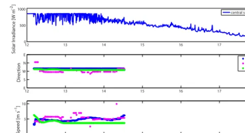
Figure 6. Solar irradiance and CMVs from CSS, USI, and LCE for
23 July. Luminance measurements of the central TEPT4400 sensor
were calibrated against a colocated pyranometer to obtain W m−2
of solar irradiance.
4 Results and discussion
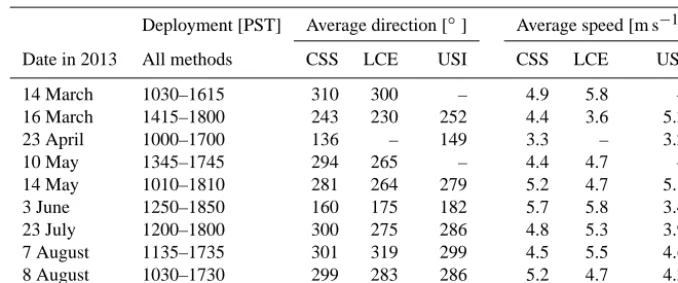
The predominant cloud conditions in coastal southern Cali-fornia are overcast stratocumulus and few to scattered cumu-lus clouds. Table 2 shows the average cloud directions and speeds on the nine deployment days. Table 3 presents the cor-responding root-mean-square difference (RMSD) and mean bias (MB).
The 23 July and 8 August deployments are selected for dis-cussion in greater detail. The KNKX METAR station 9 km to the east reported the following conditions: the air temper-ature during the 23 July and 8 August deployments was 22– 26◦C and 24–25◦C, respectively. Surface winds were 260 to 310◦ at 4.1 to 5.7 m s−1 on 23 July and 250 to 280◦ at 3.6 to 4.6 m s−1 on 8 August. There were few clouds at 400 m below scattered clouds at 900 to 1200 m a.g.l. on 23 July and few clouds at 460 m a.g.l. on 8 August.
3 June 1250–1850 160 175 182 5.7 5.8 3.4
23 July 1200–1800 300 275 286 4.8 5.3 3.9
7 August 1135–1735 301 319 299 4.5 5.5 4.6
8 August 1030–1730 299 283 286 5.2 4.7 4.3
Table 3. RMSD and MB of CSS results compared to LCE and USI. Due to incorrect cloud height observed, no cloud motion results were
detected from USI on 14 March and 10 May. LCE results are excluded for 23 April due to a shortage of results that pass QC.
RMSD MB
Direction [◦] Speed [m s−1] Direction [◦] Speed [m s−1]
Date in 2013 LCE USI LCE USI LCE USI LCE USI
14 March 41 – 3.0 – 8 – -0.7 –
16 March 25 24 0.9 1.3 −8 −8 0.9 −0.9
23 April – 20 – 0.6 – −13 – 0.1
10 May 38 – 1.5 – 31 – −0.6 –
14 May 24 20 0.9 2.5 13 1 0.4 −0.4
3 June 20 26 0.6 2.4 −15 −22 −0.2 2.2
23 July 35 14 1.2 1.2 25 14 −0.4 0.9
7 August 41 7 1.4 2.1 −18 2 −1.0 −0.2
8 August 37 26 1.3 0.9 13 13 0.4 −0.2
All 33 22 1.5 1.9 9 −0.7 −0.1 0.2
10 11 12 13 14 15 16 17 18
0 500 1000
Solar Irradiance [W m
−2]
central sensor
10 11 12 13 14 15 16 17 18
E S W N E
Direction
CSS LCE USI
10 11 12 13 14 15 16 17 18
0 2 4 6 8
Speed [m s
−1]
PST [h]
Figure 7. Solar irradiance and CMVs detected during the CSS
de-ployment on 8 August 2013.
area). Overcast conditions cause insufficient solar variability to pass the QC criteria, but the 30 min median filter causes CMV to persist into the overcast period, like during 14:00– 14:30 PST. The CSS QC directions indicate cloud movement
from the west-northwest (WNW, 300◦) direction, consistent with surface winds and visual inspection of sky imagery. USI and LCE results show an average cloud motion direction of 286 and 275◦ with RMSDs of 14 and 35◦, respectively. The CSS cloud speed ranges from 3.0 to 6.0 m s−1. USI and LCE yield an average cloud speed of 3.9 and 5.3 m s−1, with RMSD of 1.2 and 1.2 m s−1compared to CSS results, respec-tively.
and LCE with RMSD of 0.9 and 1.3 m s−1, respectively. It is
worth noting that all speed results are similar during periods of high solar variability (14:45–16:00 PST), which indicates more robustness during favorable cloud conditions. Although the three methods slightly differ in both detected direction and speed, the results lie within the range of CSS, USI, and LCE method uncertainty. True cloud speeds are not available and it is therefore unclear which sensor is more accurate.
The post-analysis conducted on days presented in Tables 2 and 3 assumes a single layer of cloud movement. In the pres-ence of multilayer clouds, several regions with high density of CMVs can be found at different cloud velocities. By using a histogram peak-finding technique on CMV results, the CSS can determine multilayer cloud movement. This method was based on prior research on CMV determination from ground irradiance data and requires further analysis, but should be feasible to implement in the CSS algorithm for identifying multilayer CMVs. Cloud motion experiencing wind shear can have a vertical speed component that is undetectable by the CSS. However, the CSS will detect 2-D cloud shadow motion (x–y plane) in scenarios with 3-D cloud movement. While this measurement may not be as useful for meteoro-logical models, the cloud shadow speed is more relevant to provide for solar variability and forecasting applications.
The analysis presented in Tables 2 and 3 also shows com-parable results between CSS, USI, and LCE results for a wide range of cloud directions (southeasterly to northwest-erly). The range of cloud speeds is more limited due to the low cloud heights and benign weather conditions in coastal southern California, but results are again consistent with the other methods. Overall speed and direction biases are essen-tially zero and typical RMSDs are 2 m s−1and 30◦.
5 Conclusions
Nine phototransistors arranged in a semicircular formation were used to obtain cloud shadow motion vectors by find-ing the maximum signal cross correlation between the differ-ent pairs of sensors. Fast sampling rates by the microproces-sor allowed the system to be compact yet able to detect the full range of typical cloud speeds from 1 to 15 m s−1(with 1 m s−1precision) and up to 24 m s−1with 2 m s−1precision. The CSS was validated using an artificial shading test appa-ratus and was found to detect cloud directions and speeds to within 15◦and 6 % accuracy, respectively. Nine deployments on partly cloudy days resulted in cloud directions and speeds consistent with those observed from a sky imager and com-puted from the LCE method.
Unlike the prior proof of feasibility in Bosch et al. (2013), the present CSS system is self-contained and more economi-cal while still producing accurate cloud motion vectors. With the present QC criteria, the CSS does not provide CMV re-sults under uniform overcast conditions, but the small solar irradiance variability in overcast conditions does not present
a major issue for solar power integration. Further optimiza-tion of the algorithm will refine QC procedures to retain as many CMVs as possible while ensuring robustness of the re-sults.
Acknowledgements. This work was supported by the California Energy Commission Energy Innovations Small Grant (EISG) and the California Public Utilities Commission California Solar Initiative RD&D programs. We are grateful to Tyler L. Capps, Andy Chen, and Jeff Head for assisting with hardware and software development; Nick Busan for providing access to the experimental facility; and (iii) Ben Kurtz, Andu Nguyen, Bryan Urquhart, and Elliot Dahlin for constructing and operating the UCSD sky imager.
Edited by: S. Malinowski
References
Arias-Castro, E., Kleissl, J., Lave, M., Schweinsberg, J., and Williams, R.: A Poisson model for anisotropic solar ramp rate correlations, Sol. Energy, 101, 192–202, 2014.
Bosch, J. L. and Kleissl, J.: Cloud motion vectors from a network of ground sensors in a solar power plant, Sol. Energy, 95, 13–20, 2013.
Bosch, J. L., Zheng, Y., and Kleissl, J.: Cloud velocity estimation from an array of solar radiation measurements, Sol. Energy, 87, 196–203, doi:10.1016/j.solener.2012.10.020, 2013.
Chow, C. W., Urquhart, B., Kleissl, J., Lave, M., Dominguez, A., Shields, J., and Washom, B.: Intra-hour forecasting with a total sky imager at the UC San Diego Sol. Energy testbed, Sol. Energy, 85, 2881–2893, doi:10.1016/j.solener.2011.08.025, 2011. Coimbra, C., Kleissl, J., and Marquez, R.: Overview of solar
fore-casting methods and a metric for accuracy evaluation, in: Solar Resource Assessment and Forecasting, edited by: Kleissl, J., El-sevier, Waltham, Massachusetts, 2013.
Hammer, A., Heinemann, D., Lorenz, E., and Lückehe, B.: Short-term forecasting of solar radiation: a statistical approach using satellite data, Sol. Energy, 67, 139–150, 1999.
Hinkelman, L., George, R., Wilcox, S., and Sengupta, M.: Spatial and temporal variability of incoming solar irradiance at a mea-surement site in Hawaii, in: 91st American Meteorological So-ciety Annual Meeting, 23–27 January 2011, Seattle, WA, United States, 2011.
Jiang, H., Xue, H., Teller, A., Feingold, G., and Levin, Z.: Aerosol effects on the lifetime of shallow cumulus, Geophys. Res. Lett., 33, L14806, doi:10.1029/2006GL026024, 2006.
Lave, M. and Kleissl, J.: Cloud speed impact on solar variability scaling – application to the wavelet variability model, Sol. En-ergy, 91, 11–21, doi:10.1016/j.solener.2013.01.023, 2013.
Lave, M., Kleissl, J., and Stein, J.: A Wavelet-based
Variability Model (WVM) for solar PV powerplants,
IEEE Transactions on Sustainable Energy, 99, 501–509, doi:10.1109/TSTE.2012.2205716, 2012.