www.atmos-meas-tech.net/7/1443/2014/ doi:10.5194/amt-7-1443-2014
© Author(s) 2014. CC Attribution 3.0 License.
The backscatter cloud probe – a compact low-profile autonomous
optical spectrometer
K. Beswick1, D. Baumgardner2, M. Gallagher1, A. Volz-Thomas3, P. Nedelec4, K.-Y. Wang5, and S. Lance6,7 1University of Manchester, Manchester, UK
2Droplet Measurement Technologies, Boulder, CO, USA
3Forschungszentrum Jülich GmbH, Institut für Energie und Klimaforschung 8: Troposphäre, 24525 Juelich, Germany 4CNRS Laboratoire d’Aérologie, Univerity of Toulouse, Toulouse, France
5Department of Atmospheric Sciences, National Central University, Chung-Li, Taiwan
6Earth System Research Laboratory, National Oceanic and Atmospheric Administration, Boulder, CO, USA 7Cooperative Institute for Research in Environmental Sciences, University of Colorado, Boulder, CO, USA Correspondence to: D. Baumgardner ([email protected])
Received: 16 June 2013 – Published in Atmos. Meas. Tech. Discuss.: 16 August 2013 Revised: 17 March 2014 – Accepted: 31 March 2014 – Published: 23 May 2014
Abstract. A compact (500 cm3), lightweight (500 g), near-field, single particle backscattering optical spectrometer is described that mounts flush with the skin of an aircraft and measures the concentration and optical equivalent diameter of particles from 5 to 75 µm. The backscatter cloud probe (BCP) was designed as a real-time qualitative cloud detector primarily for data quality control of trace gas instruments de-veloped for the climate monitoring instrument packages that are being installed on commercial passenger aircraft as part of the European Union In-Service Aircraft for a Global Ob-serving System (IAGOS) program (http://www.iagos.org/). Subsequent evaluations of the BCP measurements on a num-ber of research aircraft, however, have revealed it capable of delivering quantitative particle data products including size distributions, liquid-water content and other information on cloud properties. We demonstrate the instrument’s capabil-ity for delivering useful long-term climatological, as well as aviation performance information, across a wide range of en-vironmental conditions.
The BCP has been evaluated by comparing its measure-ments with those from other cloud particle spectrometers on research aircraft and several BCPs are currently flying on commercial A340/A330 Airbus passenger airliners. The design and calibration of the BCP is described in this arti-cle, along with an evaluation of measurements made on the research and commercial aircraft. Preliminary results from more than 7000 h of airborne measurements by the BCP on
two Airbus A340s operating on routine global traffic routes (one Lufthansa, the other China Airlines) show that more than 340 h of cloud data have been recorded at normal cruise altitudes (> 10 km) and more than 40 % of the > 1200 flights were through clouds at some point between takeoff and land-ing. These data are a valuable contribution to databases of cloud properties, including sub-visible cirrus, in the upper troposphere and useful for validating satellite retrievals of cloud water and effective radius; in addition, providing a broader, geographically and climatologically relevant view of cloud microphysical variability that is useful for improv-ing parameterizations of clouds in climate models. Moreover, they are also useful for monitoring the vertical climatology of clouds over airports, especially those over megacities where pollution emissions may be impacting local and regional cli-mate.
1 Background
trum Jülich, and in collaboration with Airbus and commer-cial carriers, has developed several miniature modular in-strument packages for commercial Airbus A330/A340 pas-senger aircraft. These modular, expandable platforms cur-rently include measurements of aerosol particle concentra-tions, reactive and greenhouse gases and, the focus of this article, cloud particle concentrations. Whilst the scientific community has learned a great deal about cloud microphys-ical processes and cloud radiative effects over the last few decades, most of the current global cloud data sets are ei-ther in situ measurements from short-term field experiments or remote-sensing data products, for example, ISCCP, (Inter-national Cloud Satellite Cloud Climatology Project) estab-lished in 1982 as part of the World Climate Research Pro-gram. Currently the data products available to the commu-nity include cloud amount, cloud type and cloud top temper-ature as well as optical thickness based on radiance. More specific retrieved microphysical properties include effective liquid-water and ice-crystal particle radius which have been validated against a wide range of WCRP and GEWEX field campaigns (e.g., GEWEX Cloud System Study Data Integra-tion for Model EvaluaIntegra-tion (GCCS-DIME) program). Typical uses for such global cloud data products are described by Rossow et al. (2005), who use cluster analysis techniques to investigate links between multi-variate relationships between clouds, mesoscale meteorological processes and global and regional energy–water budgets. Such studies are normally constrained to large fields of view and the inherent variability on sub-satellite, sub-grid scales are lost. Field campaigns to study these sub-grid scale processes, however, are expensive and time consuming to mount and are often time limited. In this respect a continuous, real-time, in situ observing system can make a contribution by providing key data products.
Commercial aircraft are limited in the types of clouds that they can sample, for example, convective cells that they would normally try to avoid or low lying, marine stratiform clouds. They do, however, fly most of their time at altitudes where they encounter many types of cirrus, a cloud type that is important for climate modulation and that can sometimes be difficult to measure with satellites. In addition, although they do not do vertical profiles of clouds, such as those done with research aircraft, their take offs and landings are often through a variety of cloud types.
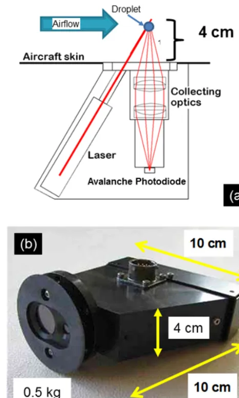
Figure 1. The optical layout of the backscatter cloud probe (BCP)
is shown in the top panel illustrating the principal components. The lower panel is a photograph of the BCP that shows the relative di-mensions.
2 The backscatter cloud probe 2.1 Design and operating principals
Figure 2. This photograph compares the backscatter cloud probe
(BCP) with the forward scattering spectrometer probe (FSSP) and the cloud droplet probe (CDP) that were introduced 38 and 12 years ago, respectively.
The collection angles were determined by the geometry of the system that was designed to keep the laser as close to the collection optics as possible so that the overall package would remain small. The sensitive sample area of the beam, as well as the collection angles, is determined by the width of the laser beam at the center of focus of the optics and the diameter of the lens.
The photons that strike the APD are converted into a cur-rent that the signal conditioning electronics change to a volt-age signal. These electronics also filter electronic noise and remove offsets due to capacitance in the electronic circuit. When the transient signal exceeds the minimum threshold, set just above the electronic noise level the peak voltage is de-tected and digitized by a 4096 bit analog to digital converter. Particles whose peaks exceed the range of the amplifiers are rejected. The value of this peak is used to select which size channel to increment by one count. The thresholds of these channels are set based upon calibrations and theory. In addi-tion to creating the size distribuaddi-tion of ADC, various voltages and temperatures, “housekeeping” parameters, are measured for monitoring the health of the instrument. The size distri-bution and housekeeping parameters are transmitted serially when given a command by a data system. The sampling rate is determined by the data system that sends the flag to the BCP to transmit the data. The BCP can be programmed to generate 10, 20, 30 or 40 channel size distributions
The compact, simple design of the BCP optical head, which weighs only 500 g and takes up a volume of less than 500 cm3, allows it to be mounted easily. Thousands of hours of flying on commercial aircraft show that it requires infre-quent maintenance. Figure 1b is a photo of the the BCP and Fig. 2 shows the BCP compared to two other single particle optical spectrometers; the cloud droplet probe (CDP), which was introduced in 2002, and the forward scattering spectrom-eter probe (FSSP), developed in 1976. This comparison illus-trates how state of the art optics and electronics has allowed
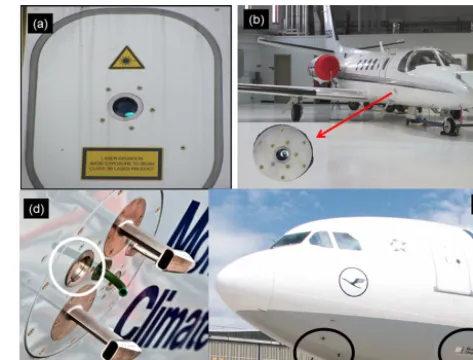
Figure 3. The backscatter cloud probe (BCP) is mounted with its
window looking out through a transparent aperture as illustrated in these four photos, clockwise: (a) on an access hatch of the FAAM BAE-146; (b) on a hard point just behind the co-pilot and just ahead of the emergency exit of the University of North Dakota Cessna Ci-tation, inside the radio compartment; and (c) on a Lufthansa A340-300 Airbus just behind and below the forward passenger access door – (d) a close-up photo of the BCP window on the Airbus.
the scaling down in size and weight of cloud spectrometers. One of the disadvantages of the BCP is that the laser is not eye-safe and so precautions are needed so as not to operate it under conditions where it could be a potential hazard. The next generation BCP, under development, will use an eye-safe laser.
The BCP mounts on the aircraft interior looking out through a transparent aperture. Figure 3 shows several pho-tos of BCP installations on the hatch of the Facility for Air-borne Atmospheric Measurements (FAAM) BAE-146, on the nose of the University of North Dakota Citation and near the nose of the Lufthansa “Veirsen” A340-300 Airbus. A pres-surized bulkhead is not required as the instrument is designed to operate up to 20 km altitude,±60◦C and 100 % humid-ity. The optical head and processing electronics are separate units connected by a cable. Interfacing to the data logger is via a standard RS-232 serial cable. The BCP can operate on 110/220 AC or 24V DC.
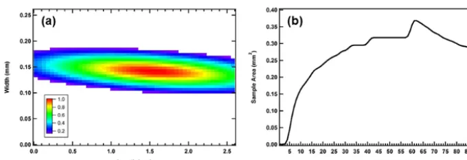
Figure 4. (a) This contour plot shows the normalized scattering intensity across the sensitive sample area of the backscatter cloud probe
(BCP). The contours values are the ratio of scattering intensity to the maximum value. (b) The sample area as a function of droplet diameter is shown in this figure.
presence of a cloud but also provides additional information about the cloud microphysical properties via distributions as a function of size of number and mass concentrations. 2.2 Calibration
The BCP sample area is measured using the calibration sys-tem described by Lance et al. (2010), which generates a highly mono-disperse droplet stream using a piezo-electric droplet generator device and transmits the droplets across precise locations of the BCP laser beam. The BCP response characteristics are mapped by moving the calibration system relative to the instrument using linear translation stages with differential positioning precision of 10 µm. The maximum light scattering intensity registered by the BCP is monitored. An intensity map is created by rastering along and across the laser beam such as the one shown in Fig. 4a. This color map is a normalized, two-dimensional Gaussian fit to the 52 measurements. The colors represent the relative intensity of scattering from the particles, where red is maximum and blue is minimum. The scattering intensity at each grid point was divided by the maximum scattering intensity to produce the normalized values. The mapping of the beam also provides a measure of the sensitive sample area of the BCP. The area is derived by summing the total number of grid points in the scan. The sensitive area for the 22 µm droplets that were used to map the beam was 0.25 mm2. The sample area de-pends on the size of the droplet, i.e., smaller droplets will be detected within a smaller area than larger droplets because of the intensity distribution of the laser beam. Ideally, each BCP should have its beam scanned using the full size range of droplets that can be measured. This might be possible us-ing a fully automatic scannus-ing system, but the current sys-tem requires manual operation and mapping from 5–75 µm, the current size range of the BCP, would require many days. Hence, the size dependent sample area can be estimated us-ing the sus-ingle map of normalized intensity values. Each grid point represents what fraction of the maximum light would be scattered by a droplet when passing through region of the beam represented by that grid point. For example, if a 10 µm
droplet scattered a maximum amount of light at the center of the beam of 3000 analog to digital counts (ADC), then far-ther away from the center, it might go through a part of the beam where it would only scatter 50 % of the maximum, or 1500 ADC. As long as the intensity of scattered light is above noise level, 50 ADC in the case of the BCP, the droplet will be detected, albeit undersized. Figure 4b shows the sample area as a function of the droplet diameter. These areas were calculated by converting the theoretical scattering cross sec-tion of a droplet of a specific size, derived with Mie (1908) theory, to equivalent ADC, derived from calibrations. These ADC were multiplied by the normalized fraction of maxi-mum scattering at each grid point. If the result of the multi-plication was greater than 50 then the area of this grid point was added to the total to produce the final sample area for that diameter of droplet.
The droplet diameter is derived from the “glare” technique (Korolev et al., 1991; Wendisch et al., 1996; Nagel et al., 2007), in which specular reflections off the front and back face of droplets are observed by a camera. These droplets of known diameter are used to to calibrate the BCP for size using Mie (1908) theory. The scattering cross section pro-vides the relationship between the voltage,V0, produced by the photodetector and associated electronics, and the scat-tered light intensity,I0. The scale factorS=I0/V0 is used to calculate scattering cross sections from the measured peak voltages. The value ofV0 is obtained when the calibration water droplet passes through the maximum beam intensity.
The intensity distribution across and along the diode laser beam is approximately Gaussian such that when a particle passes through the beam, within the viewing volume that is defined by the collection optics, it has the probability of pass-ing through different beam intensities (i.e., particles with the same optical diameter can scatter different amounts of light due to the intensity variation).
In a cloud with a range of droplet sizes, the measured size distribution will represent the sum of the probability distribu-tions of each particle size category determined by the prob-abilities that a particle will pass through a specific intensity region of the beam. Given that we have an accurate measure-ment of the intensity distribution across the sensitive beam area, we are faced with the classic inversion problem of es-timating the actual size distribution from that which is mea-sured.
2.3 Size distribution retrieval by inversion
The derivation of size distributions from the backscatter mea-surement involves the procedure, best known as inversion, in which we assume that the operating principle of the measure-ment system is well known and can be modeled such that we can predict how it will reproduce the actual size distribu-tion. Mathematically, the actual size distribution, withnsize bins, is represented by the row vectorA. The measured size distribution, with msize bins is represented by the column vector, M. Then×mmatrix, T, is a probabilistic descrip-tion of how the instrument will actually measure a particle of size i. Stated differently, the matrix T describes the proba-bility that a particle in size elementiwill actually be placed by the measurement into size elementj, where j≤i. The relationship betweenAandMis expressed as
M=TA. (1)
This is solved analytically by multiplying both sides of Eq. (1) by the inverse of T, T−1:
T−1M=T−1TA=A. (2)
This can be done only if the inverse of T can be calculated, an operation that is not usually possible in problems such as the one being posed in this application. The alternative solu-tion is to implement an iterative process in which we propose a value for the actual distribution, calling itA∗, multiply it by our transformation matrix, T, and obtain a size distribu-tion, M∗, that we compare with our measured distribution, M. IfM∗=M, thenA∗=A. Otherwise we need to adjust our value ofA∗and recalculateM∗. We continue this itera-tion until we obtain anM∗that is a reasonable approxima-tion toM (i.e., when the difference between the two vectors is within a preset value).
In order to converge on the best estimate ofA, we need an efficient method for making the first guess ofA∗and adjust-ing each subsequent guess. There are a number of problems
that must be addressed when implementing an inversion al-gorithm, for example the size distribution that can produce what is measured may not be unique, the iterative process might converge on a solution that produces a physically un-realistic distribution or our model of the system might not be sufficiently accurate. The inversion methodology is the subject of numerous articles and books related to deriving atmospheric properties from remote sensors like satellites and other types of multi-wavelength photometers. Probably the best known methodology in the atmospheric sciences is that described by Twomey (1977) for the inversion of multi-wavelength satellite measurements to obtain the properties of aerosols. To derive the size distribution measured by the BCP, we have selected a modified version of the Twomey algorithm developed by Markowski (1987).
The BCP creates the measured size histogram with m channels spanning a nominal optical diameter range from 5 µm to 75 µm, over fixed time intervals. The thresholds of the size bins are related to the peak measured voltage of the particles and are selected so that the width of the bins are approximately equal with respect to the optical diameter of the particles. The firmware in the BCP decides into which bin the particle’s peak voltage should be classified and incre-ments the bin by one so that at the end of the time interval there is a frequency distribution of the number of particles counted per size interval. This is the measured distribution, M.
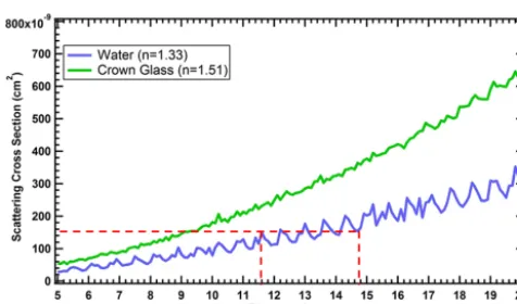
In order to create the transformation matrix, T, we need the probability distribution that predicts which fraction of the particles that fall in binj should have actually been placed in binI, as a result of the Gaussian intensity distribution of the laser beam. We also have to take into account that some particles with different sizes have the same scattering cross section due to the light scattering properties. As illustrated in Fig. 5, the scattering cross section, calculated here with Mie theory (Mie, 1908), does not increase monotonically with di-ameter. When the BCP measures the light scattered by par-ticles in some size ranges, they will be classified in smaller size intervals, as shown in Fig. 5 by the horizontal line that crosses the curve at multiple points that represents the scat-tering cross section of droplets of multiple diameters. This response must also be part of the model and included in the transformation matrix.
There are other properties of cloud particles that further complicate the derivation of size distribution, for example non-spherical ice crystals will scatter light quite differently although their geometric size might be approximately the same as a water droplet of equivalent diameter. Although these properties could be included in the matrix, T, at present we derive the transformation matrix only for the case of spherical particles with a refractive index of 1.33 (water).
Figure 5. The theoretical response of the backscatter cloud probe is
shown in this diagram that relates the scattering cross section of particles to their diameter, calculated from Mie theory assuming spherical particles, a wavelength of 685 nm and the refractive in-dices for water (1.33) and crown glass calibration beads (1.51). The red dashed line indicates an example where two particles with dif-ferent diameters have the same scattering cross section and cannot be uniquely identified by their light scattering intensity.
normalized intensity map of the laser beam in order to de-termine into which size cells,j, a particle of size,I, will fall. This produces a T matrix that is 85 rows bymcolumns. Fig-ure 6 shows the probability distributions for particles with optical diameters 10, 20, 30 and 40 µm. What is shown is the probability that a particle with the given diameter will actu-ally be classified into a smaller size category. For example, the 40 µm particle has the highest probability of being put into the 12 µm size category. Some fraction of the 40 µm par-ticles will also be classified as other diameters between 5 and 40 µm.
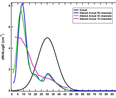
Figure 7 illustrates how the measurement with the BCP is a distortion of the actual distribution, M∗. In this figure, a theoretical Gaussian size distribution, A, is generated then multiplied by the transformation matrix, T, to calculate the hypotheticalM. The three curves in blue, green and magenta illustrate simulated size distributions assuming 90, 30 and 10 channels, respectively.
2.4 Error analysis
The BCP’s primary function when it was designed was to identify the presence of cloud. Here we define a cloud in terms of the optical depth that can be derived from the ex-tinction coefficient,Bext. This is approximated from the mea-sured size distribution:
Bext=π 6θextN (di)di2∼=π2NTda2, (3) whereθextis the extinction efficiency at a given wavelength, diameter and refractive index andN (di)is the number
con-centration of cloud particles with an optical diameter of di.
For optical diameters much larger than the incident wave-length, as will be the case for the measurements with the BCP
Figure 6. This figure illustrates the theoretical probability
distribu-tions for droplets with four different diameters. The probabilities are that a particle with the given size will be measured as a particle with a smaller diameter.
whose laser wavelength is 658 nm, the value of the extinction efficiency is approximately two. We estimate the extinction coefficient from Eq. (3) asBext=π2NTda2, whereNT is the
total number concentration anddais the area equivalent di-ameter.
Studies of cirrus in the last 10 years have led to the cate-gorization of sub-visible clouds as those with optical depth,
τ, less than 0.03 (Sassen et al., 1989). Since the BCP’s first mission is on commercial airliners whose cruise altitudes are at temperatures where only cirrus will be found, we will use 0.03 as an operational definition of a cloud to estimate the minimum concentration of cloud particles that we expect the BCP to detect. The optical depth is defined as the average extinction coefficient multiplied by the depth of the average cloud layer,1Z:
τ=Bext1Z∼=π2NTda21Z. (4)
Under the assumption of an average, area equivalent diam-eterdaand cloud depth,1Z, we can determine the number concentration of a cloud with τ=0.03. For example, thin cirrus have effective diameters in the range 30–40 µm (e.g., Gayet et al., 1996). If we chooseda=40 µm and use a con-servative value for1Z=100 m, thenBext=3×10⁻⁶cm−1 andNT =0.03 cm−3.
The concentration derived from the BCP measurements is determined by counting the number of cloud particles de-tected within the size range of the BCP over a selected time period and dividing by the volume of air,V, which passes through the sensitive sample area, SA. The volume of air is calculated as
Figure 7. The distortion of the actual size distribution due to the
measurement principles of the BCP are illustrated in this figure that shows a simulation of how the measured size distribution would appear to the BCP if the actual distribution (black curve) was cate-gorized into 90 (blue), 30 (green) or 10 (magenta) size bins.
TAS is the true airspeed at the BCP sample area andT is the sampling time. The counting efficiency of the BCP is 100 % as long as there are no coincident particles in the beam since they would be counted as a single particle. Given the very small sample area of the BCP this is a very low probabil-ity event unless concentrations exceed 500 cm−3. The prob-ability that two droplets will be in the sensitive sample vol-ume simultaneously can be estimated using Poisson statis-tics. The probability of two droplets in the sample area, SA, at the same time isP =1−e−τ λ(Baumgardner et al., 1985), whereλ=N·SA·TAS.N is the droplet number concentra-tion andτ is the amount of time that a droplet spends in the BCP laser beam, that is, the beam width (average 0.1 mm) divided by the TAS. In the absence of coincidence or other counting errors, λ is the counting rate in units of droplets per second. For example whenN=500 cm−3, for droplets of diameter 10 µm, 20 µm and 30 µm, with sample areas of SA = 0.17 mm, 0.24 mm and 0.28 mm (see Fig. 4b), the prob-abilities of coincidence are 0.8, 1.4 and 1.7 %, respectively. This would be for a BCP onboard a commercial aircraft with a cruise speed of 250 m s−1.
Hence, the source of most of the uncertainty associated with deriving the number concentration is in the determina-tion of SA and AS. The SA, as previously discussed, is mea-sured with the droplet mapping system with a linear position accuracy of±10 µm, which means that the area is estimated with a root sum square (RSS) accuracy of±14 µ m2, or±6 % for a 22 µm with sample area of 0.25 mm2.
The air speed at the sample area is the other variable needed to calculate the sample volume. The sensitive region of the BCP is 4 cm from the skin of the aircraft; hence, the
velocity of the particles at this point will likely be slower than free airstream. Aircraft airspeed sensors, however are 6 cm from the skin, so if we use the measured aircraft speed in our calculations, we estimate that an uncertainty of approxi-mately−20 % of the actual airspeed at the sample volume. In summary, the majority of the uncertainty in the derivation of the number concentration is in the sample area and airspeed. The root sum squared expected uncertainty is±21 %.
The other factor to take into account when estimating the concentration is the amount of time required to obtain a sta-tistically significant sample. Using Poisson sampling the-ory, in order to be confident that the sample is representa-tive of the general particle population, at least 100 particles must be measured to assure an uncertainty less than 10 % (n1/2/n). To measure a concentration of 0.03 cm−3, the ap-proximate concentration of a thin cirrus with an optical depth of 0.03, a volume of air of 3000 cm3must be sampled. The BCP discussed in this paper has an average sample area of approximately 0.25 mm2 and a commercial airliner flies at an airspeed of approximately 250 m s−1. This means that 63 cm3s−1of air is sampled and measurements would need to be accumulated over approximately 45 s to obtain a sta-tistically relevant value. If a 20 % uncertainty is acceptable, then only 25 particles are needed and the sampling time is reduce to 10 s.
The accuracy with which the actual size distribution is de-rived is a function of five factors: (1) the number of channels in the measured size distribution, (2) the fraction of the ac-tual size distribution with concentrations in optical diameters smaller than about 15 µm, (3) the width of the actual distri-bution, (4) the refractive index of the particles and (5) their shape. The accuracy depends upon how much of the original information contained in the actual distribution is maintained during the measurement process. The particles are being un-dersized over a range of values as they go through the sample area in uniformly, random locations. If they are placed in a smaller size bin, whose width is very small, then the new size has retained most of the original information. For example if a 20 µm particle gets sized some of the time as a 10 µm par-ticle, and if the width of the channel for 10 µm particles is only 1 µm, then the inversion will put that particle back into the 20 µm bin. If the width of the channels in the measured distribution is 5 µm, the information is lost when the 20 µm particle gets sized as a 10 µm particle. In the process of re-binning it is placed in a channel that might also contain 7, 8, 9, 10, 11, and 12 µm particles. In this case, the inversion will be unable to produce as accurate of a representation of the actual distribution since 7–12 µm particles can end up in the size bins around the 20 µm size bin of the retrieved distribu-tion. The subsequent effect is a retrieved distribution that is broader than the actual.
Figure 8. The three panels illustrate how the accuracy of retrieving the actual size distribution is related to the width of the distribution. The
black curve is a simulated distribution with an average diameter of 20 µm and standard deviation of 2 µm, 6 µm and 10 µm in panels (a), (b) and (c) respectively. The blue curves are the distributions retrieved from the simulated measurements shown in green and the red curve shows the predicted measurement after the inversion.
lost when they go through the edges of the beam. Hence, in-formation from the actual distribution is lost from the small particle sizes that cannot be completely retrieved since we do not know a priori what the shape of the actual distribution will be.
The third parameter that limits the accuracy of the retrieval is the width of the actual size distribution. This is also an is-sue of information loss. The most rigorous test of a retrieval is that of a mono-dispersed particle distribution whose mea-sured distribution would look similar to one of the probabil-ity distributions that were shown in Fig. 6 if the channels of the measured distribution have very narrow widths so as to capture the detailed structure of the many possible measured sizes. Due to the finite widths of the measured distributions, however, these structures are smoothed out so that the subse-quent inversion produces a retrieved distribution broader than mono-dispersed. When the actual distribution is broader, the resultant distribution that is measured is the mixture of prob-abilities that also smooth the intrinsic shape of the proba-bility distributions. The retrieval is able to better reproduce the broader actual distribution as illustrated in Fig. 8. Here the actual distribution is simulated with a Gaussian proba-bility distribution with a constant concentration and average diameter of 100 cm−3and 20 µm, respectively. The standard deviations are set to 2 µm, 6 µm and 10 µm. The black curves are the simulated actual distributions; the green curves are the simulated “measured” distributions, assuming a 90 chan-nel simulated “measured” distribution. The simulated “mea-sured” distribution is similar to that illustrated in Fig. 6 where the simulated actual distribution is multiplied by the transfor-mation matrix. The blue and red curves show the simulated actual and “measured” distributions following application of the inversion.
Figure 9 shows the result of evaluating a range of simu-lated actual and “measured” size distributions. The number of channels of the simulated measured distributions, the av-erage diameter and the standard deviation of the distribution are varied in order to evaluate the accuracy of the retrieval with respect to the three factors discussed above. The error is
Figure 9. The sets of curves shown in this figure illustrate the
accu-racy of the inversion as a function of the standard deviation of the simulated actual (Gaussian) size distribution. Each color represents a simulated, measured size distribution binned in 10 channels (red), 30 (blue) and 90 (green). The average diameter of the simulated ac-tual distribution is varied from 10 µm (solid curves), 20 µm (dashed) and 30 µm (dot-dash).
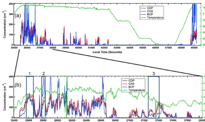
Figure 10. In this time series of cloud particle concentrations, the cloud droplet probe (CDP (black), cloud and aerosol spectrometer (CAS)
(red) and backscatter cloud probe (BCP) (blue) are compared over the entire flight of the BAE-146 on 14 September 2011 in the top panel and over the liquid-water segment of the cloud in the lower panel. The green curve is the ambient temperature. The numbered boxes are cloud segments where size spectra averages are calculated and displayed in Fig. 12.
3 Flight results
The measurements on the BAE-146, operated by FAAM, were made in September, 2010, on flights over the North At-lantic as part of the IAGOS-DS and Septex Cloud-Radiation projects (http://www.faam.ac.uk/index.php/home). Measure-ments were made through a range of cloud types and temper-atures from which one example is highlighted here. As was previously shown in Fig. 3a, the BCP was mounted on the forward, starboard window-blank no. 3 located∼5 m from the aircraft nose upstream of the aircraft’s Johnson–Williams hot-wire total liquid-water content probe. In addition to the BCP, there were other cloud microphysical optical spectrom-eters flown, including the DMT cloud droplet probe (CDP) that has been described by Lance et al. (2010) and a cloud and aerosol spectrometer (CAS) described by Baumgardner et al. (2001). The CDP, CAS and other 2-D optical array probes were mounted on the starboard wing pylons, 8 m aft of the BCP.
Figure 10a is a time series of number concentrations from the BCP, CDP and CAS during a 4 h flight (B553 using the FAAM research flight designation) conducted on 14 Septem-ber 2010. Figure 10b shows the same variables but over the time period 35 000–38 000 UTC seconds from start of the day. This was a period when the aircraft was penetrating clouds that were all liquid water. The concentrations from the CAS, that measures in the size range from 0.5 to 50 µm, and from the CDP, which measures from 2.0 to 50 µm, were cal-culated over the same size range as that of the BCP used dur-ing this project (ca. 4 to 45 µm). As previously noted, without an airspeed measurement at the location of the BCP sample
area, there is an uncertainty of approximately 20 % in calcu-lating the sample volume, that is, although we are using the recorded aircraft true airspeed to calculate the BCP sample volume, the actual volume could be as much as 20 % smaller. In the majority of the cloud passes during this 50 min pe-riod of sampling the BCP measured concentrations that were within 20 % of those derived from the CDP and CAS. During the period from 35 700 to 36 150, the BCP would occasion-ally increase to almost a factor of two greater than the other two spectrometers. During the period from 37 000 to 37 600, the BCP concentrations were about half of those from the other two instruments.
Figure 11a and b compare the liquid-water content (LWC) and optical median-volume diameter (MVD) from the three probes for the same time periods as shown in Fig. 10b. As with the concentrations, the BCP LWC is generally in good agreement with the other two spectrometers except during the same time periods where the number concentrations de-viated. The BCP MVD falls between those of the CDP and CAS except for the period from 37 000 to 37 600 when the CDP and CAS MVDs increase but the BCP MVD remains about what it had been throughout the period.
Figure 11. These time series of liquid-water content (LWC) in the top panel and optical median volume diameter (MVD) in the lower panel
are over the same interval of time as shown in Fig. 10b.
case, Fig. 12-1, the BCP size distributions falls almost on top of that from the CAS for droplet diameters larger than 10 µm and overestimates the concentration of smaller droplets. The CDP size distribution is narrower than those from the BCP and CAS. In the second time interval over which the mea-surements were averaged and in which the BCP was much higher in concentrations, we see in Fig. 12-2 that the BCP is higher in concentration over the entire size range. The CAS also exceeds the CDP over all sizes, although not to the same degree as the BCP. For the case when the BCP concentra-tions and MVDs were smaller than the CDP and CAS (time interval 3), we see from Fig. 12-3 that the peak in the size distribution from the BCP falls to the left of both of the other spectrometers. The concentrations are also much less at all sizes. It should be pointed out that the CAS and the CDP are not necessarily providing the “correct” answer and the pur-pose of these intercomparisons is to evaluate the BCP against spectrometers that have been in use for a longer period of time. As can be seen from these examples the CDP and CAS are not in perfect agreement; however, the differences remain approximately the same in all three time intervals, whereas the BCP differs in a manner that cannot be explained at this time.
Two BCPs were delivered to the IAGOS management team for installation on a Lufthansa A340-300 “Viersen” air-liner in May, 2011, along with the rest of the IAGOS instru-ment package (O3, CO, CO2, NOy, NOx, H2O). The BCP was mounted next to the inlets for the aerosol and gas ana-lyzers as shown in the photographs in Fig. 3c and d.
The first test flight of the Viersen with the IAGOS pack-age took place in July, 2011, and routine operation began in September, 2011. Additional IAGOS systems were installed on a China Airlines A340 “B-18806”, an Air France A340 “F-GLZU”, a Cathay Pacific A340 “B-HLR” and an Iberia A340 “EC-GUQ” in 26 June 2012, and June, August and
Figure 12. The size distributions shown here illustrate how the
Figure 13. The trajectories for the Lufthansa (September, 2011–March, 2013) and China Airlines (January–March, 2013) commercial flights
are shown here encoded with cloud encounters (colored, filled circles) and locations of arrivals and departures (yellow diamonds). The color scale shows the number concentrations of the clouds that were identified.
October of 2013, respectively. The BCPs on these commer-cial aircraft is sampled at 0.25 Hz and transmits ten channel size distributions. Ten channels were chosen to minimize the amount of data that were recorded and prevent filling the stor-age device. The data are recorded during several flights then routinely downloaded by IAGOS technical staff.
As of March, 2013, the BCPs had taken data on a total of 1211 flights, representing 7357 h of flight time during which 340 of those hours had been in cloud. We define a cloud as one with a number concentration greater than 0.01 cm−3 for more than 20 seconds (five samples from the BCP). Fig-ure 13 summarizes the trajectories of all the flights for the 18 months covering 1 September, 2011, to the end of March, 2013. Table 1 list some basic statistics with respect to the regions that were covered by the flights.
Figure 14 and 15 are expanded views of the flights be-tween Europe and North America and Europe and South America, respectively. These two regions are highlighted be-cause flights covering these regions are the longest in du-ration and 70 % of these flights also encountered clouds at cruise altitude. More than 90 % of the flights from Frank-furt to Rio encountered clouds at cruise altitude. The Asia routes (not shown here), although somewhat shorter in dura-tion, also encountered clouds at cruise altitude during more than 70 % of the flights.
4 Discussion
Although the BCP was originally designed as a cloud indi-cator, its design includes a method to estimate the effective optical diameter (EOD) of individual particles. The EOD is the diameter that a spherical water droplet would have if it scattered the same amount of light that was measured. The
derivation of the EOD is complicated by the Mie scattering ambiguities and the non-uniform incident laser intensity that requires an inversion of the data to derive the EOD. The size distributions from the BCP, along with the number concen-tration, LWC and MVD, were compared with two other sin-gle particle spectrometers. The BCP was generally within 20 % of the other sensors except for several time periods when it either overestimated or underestimated the bulk pa-rameters. The source of the differences cannot be explained but there are a number of possible causes.
Figure 14. Similar to Fig. 13, but expanded to show only the flights between Europe and North America.
Table 1. Cloud statistics from Airbus A340-300 BCP measurements. Number concentrations > 0.01 cm−3define a cloud.
Fraction of flights Fraction of Fraction of Total Fraction of with cloud flights with flights with Total flight Total time flight hours encounters at cloud encounters cloud encounters Region flights hours in cloud in cloud (%) cruise altitude (%) at takeoff (%) at landing (%)
Africa 85 453 34.9 7.7 62 54 61
America 128 1035 48.9 4.7 70 62 69
Asia 103 895 49.3 5.5 73 64 62
Europe 40 462 5.0 1.1 10 45 58
Far East 391 1390 53.5 3.8 24 46 53
Gulf 176 769 25.6 3.3 19 39 42
Middle East 111 462 17.2 3.7 26 42 47
Pacific 64 669 8.4 1.3 13 41 38
Rio 99 1117 97.9 8.8 94 76 80
All 1211 7357 340 4.6 40 50 55
done for various research aircraft to locate optimum mount-ing positions for cloud probes, we do not know what type of enhancements might be occurring in the concentrations at various aerodynamic diameters. At some locations on the air-craft there can also be a “shadow zone”, where the boundary layer has grown to a thickness sufficient to carry cloud par-ticles outside of the sensing volume of an instrument. This is apparently not the case for either the measurements on the BAE-146 or the Airbuses given that the BCP is detect-ing cloud particles.
Ice-crystal shattering is another source of uncertainty and measurement error. A number of studies have highlighted the issue of ice crystals shattering and water droplets splatter-ing on the leadsplatter-ing edges of instruments (e.g., Engblom and Ross, 2003; Korolev et al., 2013), leading to artificially cre-ated particles that confound the measurements. The geome-try of the BCP, that is, lack of any leading edges for droplets or crystals to impact and break, means that the instrument itself will be free of probe-induced artifact; however, the
Figure 15. Similar to Fig. 13, but expanded to show only the flights
between Europe and Rio de Janeiro.
temperatures), can sometimes grow to sizes large enough to fracture on impact.
The comparison of the BCP with the CDP and CAS on the BAE-146 was encouraging from two aspects: (1) the num-ber and mass concentrations generally compared within 20 % over the whole flight and (2) the size distributions were in good agreement with respect to peaks and shapes. This gives us confidence that a measurement so close to the aircraft skin can give a reasonable representation of the cloud properties and that the inversion technique is robust enough to extract size information.
The preliminary analysis from the BCP on the commercial passenger airliners shows an abundance of cloud data and a wealth of information that can be extracted on cloud micro-physical properties in the size range of the BCP. The caveat is that care must be taken when ice shattering may be a po-tential source of artifacts. A detailed analysis of these data is well beyond the scope of this paper where we have fo-cused on the technical aspects of the BCP. That being said, a cursory look at some of the regions of the world where desert dust and clouds are encountered offer a tantalizing hint of the types of information that can be obtained. These are data that can be used to compare with satellite measurements
Figure 16. These vertical profiles of the number concentration in
the left panel and average optical diameter in the right panel are an example of multilayered clouds (red horizontal lines) measured with the backscatter cloud probe as the aircraft was landing in Frankfurt, Germany in May, 2011. Cloud layers are delineated by the peaks in concentration greater than 100 cm−3.
and to validate climate and cloud/dust models. Looking at the flight trajectories from Frankfurt to Rio de Janeiro in Fig. 15, we see that there are many clouds and quite a few with concentrations greater than 1 cm−3 (1000 L−1). More than a 1000 L−1is an enormously high concentration of ice crystals for cirrus, the type of cloud that would normally be found at these altitudes and temperatures. Such large concen-trations have been measured (Jensen et al., 2013); however, it is more likely that the ice-crystal concentration is being mul-tiplied by breakup on the fuselage. From the point of view of better understanding ice cloud microphysics, these high, arti-ficial concentrations obscure some of the important features of these clouds. From the viewpoint of aircraft flight opera-tions, such high concentrations are potential hazards as these crystals and their fragments are the very type of cloud parti-cles that have been documented as obstructing inlets to tem-perature sensors and pitot tubes that measure air speed. These measured high concentrations are found not only over the same route where documented aircraft incidents have hap-pened, but also over many other regions of the world. This underscores the importance of having this type of informa-tion available in real time for flight crews to make informed decisions.
of the BCP sample area that is obtained using measurements with a mono-dispersed droplet stream.
The comparison of the BCP with two other spectrometers, the CDP and CAS, show that the BCP, whose active sample volume is only 4 cm from the aircraft skin, generally agrees within 20 % in number concentration and size distributions measured with the other two spectrometers.
The BCPs on two commercial airliners, Lufthansa and China Airlines Airbus A340-300s, have taken more than 7000 h of data during more than 1200 h of flight time. At a cruise altitude between 9 and 11 km, 40 % of the flights en-countered cirrus and 50 % of the take offs and landing were made through cloud layers. The 340 total hours of cloud data and more than 600 vertical profiles through cloud are a valu-able database of information that provide measurements that can complement those from remote sensors like radar, lidar and satellites, as well as being useful for validating algo-rithms for extracting microphysical properties from remote-sensing measurements. As with data from any cloud spec-trometer in conditions of high ice concentration, care must be taken when interpreting any data sets where ice shattering on the fuselage may produce artifacts in the measurements.
In addition to the value for research on cloud proper-ties, the data also provides important information to the air-craft industry on statistics related to the frequency of flight encounters with high-ice-crystal concentrations, events that pose potential hazards to flight operations.
Acknowledgements. The authors would like to thank the staff of
the Facility for Airborne Atmospheric Measurements (FAAM), Bill Dawson, Roy Newton and Gary Granger of Droplet Measure-ment Technologies and Lufthansa and China Airlines for their cooperation in partnering with IAGOS to make these invaluable environmental measurements. Financial support of the instrument development, installation and operation from the European Com-mission projects IAGOS-DS and IAGOS-ERI, national agencies in Germany (BMBF), France (MESR), and the UK (NERC), and the IAGOS member institutions (http://www.iagos.org/partners) is gratefully acknowledged. The calibration work was supported by the National Oceanic and Atmospheric Administration (NOAA) climate and air quality programs. Finally we would like to than David Delene and Gabor Vali for their detailed reviews that greatly improved the quality of this manuscript.
Edited by: P. Herckes
(CAPS): A new instrument for cloud investigations, Atmos. Res., 59–60, 251–264, 2001.
Engblom, W. A. and Ross, M. W.: Numerical Model of Airflow In-duced Particle Enhancement for Instruments Carried by the WB-57 Aircraft, NASA Aerospace Report No. ATR-2003(5084)-01, 29 pp., 2003.
Gayet, J. F., Febvre, G., Brogniez, G., Chepfer, H., Renger, W., and Wendling, P.: Microphysical and Optical Properties of Cirrus and Contrails: Cloud Field Study on 13 October 1989, J. Atmos. Sci., 53, 126–138, 1996.
Jensen, E. G., Diskin, G., Lawson, R. P., Lance, S., Bui, T. P., Hlavka, D., McGille, M., Pfister, L., Toon, O. B., and Gao, R.: Ice nucleation and dehydration in the Tropical Tropopause Layer, P. Natl. Acad. Sci., 110, 2041–2046, 2013.
King, W.: Air flow and particle trajectories around aircraft fuse-lages. I: Theory, J. Atmos. Ocean. Tech., 1, 5–13, 1984. King, W., Turvey, D., Williams, D., and Llewellyn, D.: Air flow and
particle trajectories around aircraft fuselages. II: Measurements, J. Atmos. Ocean. Tech., 1, 14–21, 1984.
Korolev, A. V., Kuznetsov, S. V., Makarov, Y. E., and Novikov, V. S.: Evaluation of Measurements of Particle Size and Sample Area from Optical Array Probes, J. Atmos. Oceanic Tech., 8, 514–522, 1991.
Korolev, A. V., Emery, E. F., Strapp, J. W., Cober, S. G., and Isaac, G. A.: Quantification of the effects of shattering on airborne ice particle measurements, J. Atmos. Ocean. Tech., 30, 2527–2553, 2013.
Lance, S., Brock, C. A., Rogers, D., and Gordon, J. A.: Water droplet calibration of the Cloud Droplet Probe (CDP) and in-flight performance in liquid, ice and mixed-phase clouds during ARCPAC, Atmos. Meas. Tech., 3, 1683–1706, doi:10.5194/amt-3-1683-2010, 2010.
Markowski, G. R.: Improving Twomey’s Algorithm for Inversion of Aerosol Measurement Data, Aerosol Sci. Technol., 7, 127–141, 1987.
Mie, G.: Beiträge zur Optik trüber Medien, speziell kolloidaler Met-allösungen. Annalen der Physik, Vierte Folge, Band 25, No. 3, 377–445, 1908.
Nagel, D., Maixner, U., Strapp, W., and Wasey, M.: Advance-ments in Techniques for Calibration and Characterization of In Situ Optical Particle Measuring Probes, and Applications to the FSSP-100 Probe, J. Atmos. Ocean. Tech., 24, 745–760, doi:10.1175/JTECH2006.1, 2007.
Norment, H.: Three–dimensional trajectory analysis of two drop sizing instruments: PMS OAP and PMS FSSP, J. Atmos. Ocean. Tech., 5, 743–756, 1988.
Sassen, K., Griffin, M. K., and Dodd, G. C.: Optical scattering and microphysical properties of subvisible cirrus clouds, and climatic implications, J. Appl. Meteorol., 28, 91–98, 1989.
Twohy, C. and Rogers, D.: Airflow and water drop trajectories at instrument sampling points around the Beechcraft King Air and Lockheed Electra, J. Atmos. Ocean. Tech., 10, 566–578, 1993.
Twomey, S.: Introduction to the Mathematics of Inversion in Re-mote Sensing and Indirect Measurements, Developments in Ge-omathematics 3, Elsevier Scientific Publishing Company, Ams-terdam, 237 pp., 1977.