TERRAIN CLASSIFICATION FOR
TRAVERSABILITY ANALYSIS FOR
AUTONOMOUS ROBOT NAVIGATION
IN UNKNOWN NATURAL TERRAIN
* PRIYANKA MATHUR
Department of Electronics and Communication Engineering Ansal Institute of Technology, Gurgaon, India
Email: [email protected] KK SOUNDRA PANDIAN
Department of Electronics and Communication Engineering
Indian Institute of Information Technology, Design & Manufacturing ,Jabalpur,India Email:[email protected]
Abstract
Autonomous robot navigation in unknown natural terrain is the key requirement of a robotic system such as a rover as the natural terrain is unpredictable. For safe and robust navigation a robot must possess onboard intelligence to perceive the terrain ahead so that it can avoid hazardous areas by discriminating the navigable regions for traversal thereby optimizing its speed and increasing its efficiency. This is accomplished by real-time assessment and classification of terrain for traversability analysis. In this paper terrain classification system is developed for its traversability analysis for the robot operating in natural unknown terrain. The proposed method classifies the unknown terrain describing its suitability for navigation by extracting the textural features from visual imagery of terrain data. Clustering technique is employed to classify the features derived from statistical and transform based texture analysis. And further we have presented a fast and optimum algorithm for path planning of robot on the assessed navigable terrain. Images from NASA’s Mars exploration rover and those obtained from real time natural terrain have been tested to validate the proposed approach.
Keywords: Autonomous robot navigation, real-time assessment, terrain classification, traversability analysis, path planning
1. INTRODUCTION
The purpose of this paper is to develop a terrain classification algorithm is proposed based on extracting textural features from terrain image obtained by using vision sensors. Our method identifies the terrain prior to traversing so that unsuitable terrains and obstacles could be avoided. This will enables the robot to sense its underline terrain similar to how humans determine the terrain on which they are driving.
Our approach uses the texture information derived from statistical and transform based analysis of the terrain regions. Salient features of terrain such as energy, entropy and contrast are extracted from co-occurrence matrix computed out of the sub bands of wavelet packet decomposed region of the terrain. These features form a complete feature vector which is classified by using k means clustering Furthermore; we have developed an optimum and shortest path planning algorithm for mobile robot in natural terrain similar to Mars surface terrains.
The rest of the paper is organized as follows. A review of the related research work in the area of terrain classification is given in section 2.Section 3.describes the proposed methodology for terrain classification for traversability assessment. It explains the feature extraction methods and discusses the classifier used. The details of the proposed path planning algorithm for the robot in navigable terrain are elucidated in section 4.Section 5.presents the experimental results of our traversability assessment of terrain and path planning algorithm and finally section 6.deals with the conclusion and possible extension for the future work.
2. PROLOUGE ASSESSMENT
Terrain classification methods provide semantic descriptions of the physical nature of a given terrain region. These descriptions can be associated with nominal numerical physical parameters, or nominal traversability estimates, to improve traversability prediction accuracy. Numerous researchers have proposed terrain classification methods based on features derived from remote sensor data such as color, image texture, and range (i.e. surface geometry) and vibration derived from different sensors such as laser range finder, ultrasonic range finder, vision sensor, tactile sensors Terrain traversability based on terrain classification and path planning of terrain-adaptive robots have been addressed by a number of researchers. Howard and Seraji [1] introduced the Fuzzy Traversability Index Algorithm, which used visual intensity levels to determine the terrain characteristics such as the roughness, slope, and discontinuity. Another classification method by Vandapel [2] avoids the effects of variability in light intensity by the use of statistical properties of 3D ladar sensor data to detect the surrounding terrains This method applied off-line statistical analysis techniques to ladar sensor data to segment a scene into three classes: vegetation, terrain rocks, and thin wires or tree branches. Machine learning methods were employed by D.F.Wolf [3] using 2 D laser range finders. Range information also known as geometric information, generates point clouds which are classified into navigable and not navigable area using hidden markov models (HMM). J.Soenneker et al. [4] used local point statistics features extracted from 3-D point cloud generated by ladar scans and enabled Naïve Bayes Decision Tree to learn to distinguish between different classes of terrain. In [5] Manduchi used a combination of color camera images and ladar data to detect and classify obstacles, with the detection done via ladar and classification using camera. A.Birk et al. [6] processed the range data obtained from Laser Range Finder by a Hough transform with three dimensional parameter spaces for representing planes and classified the terrain by Decision tree. However such methods cannot easily detect non-geometric hazards or terrain classes that are not characterized by variations in geometry. . Shirkhodaie et al. [8] used visual terrain modeling using soft classifiers like rule based and neural networks. Olson et al. [9] used visual stereo imaging fusion technique and demonstrated a reliable method for high fidelity terrain mapping and robot world perception modeling.
Texture analysis can also be efficiently utilized in the area of terrain classification. Dong Min et.al[15] used co-occurrence features with linear discriminate classifier and clustering algorithm based on artificial neural network for terrain classification especially for shadow, grass and road class. Texture classification itself is an image processing technique which is basically employees ed in computer vision applications, industrial automation and in content based image retrieval. Mathur P. et.al used textural gray level co-occurrence features with crisp rule based classifier to classify the terrain into several regions of navigable and not navigable area [16]
3. METHODOLOGY
3.1 System Overview
Classification of terrain consists of two stages .Initially identifying and extracting the features that could be used for achieving maximum classification accuracy and then classifying the data using classifiers We have used textural analysis on the visual imagery terrain data. Texture is a measure of the local spatial variation in image intensity .It can be characterized by different approaches such as statistical means; model based or transforms based texture analysis. Statistical method is based on various joint probabilities of gray values. Gray Level Co-occurrence Matrices (GLCM) estimates the second order statistics by counting the frequencies for all the pairs of gray values and all displacements in the input image. The major texture attribute such as energy, entropy and contrast are derived from co-occurrence matrix. Model based methods include fitting of model like Markov random field, autoregressive, fractal and others. The estimated model parameters are used to segment and classify textures. Transform based approach analyses texture in various transform domains usually implemented through various filter banks such as Gabor filter and wavelet decomposition etc.
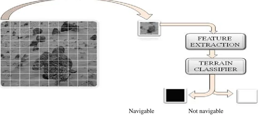
The proposed terrain classification method consists of initially dividing the terrain image into finite number of sub frames where each frame represents a small portion of the actual terrain called the sub terrainian region. Texture features are then extracted from each sub image which is fed to the classifier that classifies/renders the given sub frame into either navigable or not navigable region
Navigable Not navigable Fig. 1. Design flow of terrain classification
Fig.2. System Architecture of terrain classification 3.2 Feature Extraction
Our approach to obtain feature vector is to apply wavelet packet decomposition on each sub terrain image and the co-occurrence matrix is calculated out of the sub bands of decomposed images. Several texture measures are directly computed from the grey level co-occurrence matrix such as contrast, entropy, variance and energy. 3.3 Grey Level Co-Occurrence Matrix
Gray Level Co-occurrence Matrices (GLCM) estimates the second order statistics by counting the frequencies for all the pairs of gray values and all displacements in the input image. An image is a matrix of pixel intensities, I (i,j) We can define co-occurrence of image matrix as Pd (i,j)such as every entry in co-occurrence matrix, Pd(i,j), is difference in intensity between a pair of image pixels(i and j), that are distance d pixels apart in original image in a given direction. Energy associated with an image that is a measure of textural uniformity of an image is defined by equation (1)
=
i
d j
j
i
P
Energy
2(
,
)
(1)Furthermore, Image Entropy is a measure of disorder of an image Entropy is inversely proportional to Energy and is defined by equation (2)
−
=
i
d j
d
i
j
P
i
j
P
Entropy
(
,
)
log
(
,
)
(2)The image texture contrast measures the amount of local pixels intensity variation within an image
−
=
i j
d
i
j
P
j
i
Contrast
(
)
2(
,
)
(3)= ∑ ∑ ( , ) ( , ) − / (4) Where , , are means and standard deviations respectively of P(i,j)
We compute these features for all the sub terrain regions which serve as feature vector for the classifier and forms first feature set (FS1). In addition two more feature database is created by using wavelet statistical features which contains energy values of leaf nodes of the wavelet packet decomposed image at level 3 forming feature set 2 (FS 2) and other obtained by directly calculating co-occurrence features from the original sub image forming feature set 3 (FS 3).
Classification is done using all the three different feature databases. It is found that the success rate is improved much in our approach by combining wavelet statistical and co-occurrence matrix features of decomposed images
3.4 The Wavelet Packet Decomposition
For many signals, the low-frequency part contains the most important part. In such cases, one must pay attention in the bands of high energy, instead of looking with fine frequency bandwidths at low-frequency bands of low energy. This leads to the adoption of wavelet packets .Discrete wavelet packet transform consists of Wavelet packet decomposition (WPD) sometimes known as just wavelet packets. It is a wavelet transform where the signal is passed through more filters than the discrete wavelet transform (DWT).
Fig.3. Image decomposition (a) One-level (b) two level.
In DWT The image is actually decomposed i.e., divided into four sub-bands and critically sub-sampled by applying DWT as shown in Fig. These sub-bands labeled LH1, HL1 and HH1 represent the finest scale wavelet coefficientsi.e., detail images while the sub-band LL1 corresponds to coarse level coefficients i.e., approximation image.
Fig.4. Wavelet Packet decomposition tree
an approximation and three detail images. The approximation image is then itself split into a second-level approximation and detail images, and the process is recursively repeated. So, there are (n + 1) possible ways to decompose or encode the image for an n-level decomposition. In 2D-DWPT analysis, the three details images as well as the approximation image can also be split. So, there are 4n different ways to encode the image, which provide a better tool for image analysis.
3.5 Terrain Classifier ( K means Clustering )
A cluster is a collection of objects which are similar between them and are dissimilar to the objects belonging to other clusters. Clustering of numerical data forms the basis of various classification and system modeling algorithms. The purpose of clustering is to identify natural groupings of data from a large data set to produce a concise representation of a system's behavior. Clustering algorithms are not only used to organize and categorize data, but are helpful in data compression and model construction. In statistics and machine learning, the k-means algorithm is clustering algorithm to partition n objects into k clusters, where k < n. This technique is based on randomly choosing k initial cluster centers, or means. These initial cluster centers are updated in such a way that after a number of cycles they represent the clusters in the data as much as possible. The k-means algorithm starts with k- cluster centers or centriodes. Cluster centriodes can be initialized to random values or can be derived from a priori information. Each data point then assigned to the closest cluster (i.e. closest centriodes). Finally, the centriodes are recalculated according to the associated data. This process is repeated until convergence. Data vectors within a cluster have small Euclidean distances from one another, and are associated with one centriodes vector, which represents the "midpoint" of that cluster. The centriodes vector is the mean of the data vectors that belong to the corresponding cluster.
1. The algorithm starts out with initializing Ci this is achieved by randomly Selecting C points from among all the data points.
2. Determine the membership matrix U, where the element uij is 1 if the jth data point xj belongs to the group 1 and 0 otherwise.
3. Compute the cost function by the equation given below. Stop if the value of cost function is below a certain threshold value.
= ∑ = ∑ ∑ , ∈ || − || ( 5 )
4. Assign each data point to the cluster closest centroide
5. Update the clusters center centers Ci by re calculating the clusters centriodes as mean of all data points within the each cluster and determine the new U matrix.
4. PATH PLANNING ON ASSESSED TERRAIN
Fig.5. Path planning algorithm from source (yellow) to goal (red)
The algorithm determines the most suitable way point towards the goal in the navigable region that minimizes the number of traveling cells thereby giving the shortest path.
5. RESULTS AND PERFORMANCE EVALUATION
The performance of the terrain classifiers for traversability analysis was on two different terrain image databases. The first set was compiled from NASA’s Mars Exploration Rover mission. High resolution panoramic camera images selected from MARS Analysts Notebook database to verify the algorithm performance on MARS surface scenes. The second set of images was collected through digital camera from real time natural terrain.
Initially we divide the terrain image into finite number of sub frames. Each frame represents a small portion of the actual terrain called the sub terrain region. The images were of the size 320X 320 .We chose a sub window frames of size 32 X 32 for terrain sampling. For Mars surface scenes, primary terrain types that are believed to possess distinct traversability characteristics are: rocky terrain composed of outcrop or large rocks; sandy terrain, composed of loose drift material and smooth mixed terrain .Examples of these terrains are shown in Fig.6
Fig.6. Class Distinction of Mars terrain
contains energy values of the leaf nodes of wavelet packet decomposed image. Fig. 7 shows the classification result of the terrain image 1 (TI 1) using features of first feature set (FS1)
Fig. 7. (a) Terrain Image 1 (b) Sampled Terrain (c) Classified Terrain
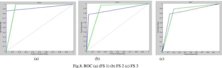
The performance of a classifier can be measured by classification accuracies and speed. Accuracy is evaluated using Receiver Operating Characteristics (ROC) curve and the confusion matrix .It summarizes how well the classifier has performed for that problem at different thresholds. It allows us to show graphically the trade off of each classifier between its true positive rate (the number of correct positive cases divided by the total number of positive cases) and its false positive rate (the number of incorrect positive cases divided by the total number of negative cases) by the total number of positive cases) and its false positive rate (the number of incorrect positive cases divided by the total number of negative cases). Here horizontal axis indicates the percentage of false positives and the vertical axis indicates the percentage of true positives. The point (0,1) is the perfect classifier as it classifies all positive cases and negative cases correctly. It is (0,1) because the false positive rate is 0 (none), and the true positive rate is 1 (all). The point (0,0) represents a classifier that predicts all cases to be negative, while the point (1,1) corresponds to a classifier that predicts every case to be positive. Point (1,0) is the classifier that is incorrect for all classifications. Thus, higher the curve is towards the left higher is the correct classification rate as vertical axis shows true positive value, its higher percentage corresponds to higher correct classification and horizontal axis showing false positive value should have minimum value therefore it should have lower percentage for less number of misclassified regions. ROC curve should lie as close to left for FPR to be nearly close to zero and TPR to be nearly close to maximum 100%.Fig. 8(a) shows the ROC curves for terrain image 1. Here,green curve is the roc for navigable classes and blue curve is roc of not navigable class.As the curve in fig. 8 (a) is highly towards the left as compared to the curve in fig. 8 (b) and 8c), it indicates that the classified output performed better using FS 1 as the true positive rate is more and false positive rate is low. In fig. 8(b) and 8(c) curve lies away from the vertical axis showing more false positive rate as compred to fig. 8 (a). Thus the classification accuracy uaing our feature set performed better Blue curve line indicates the correct positive rate for not navigable regions and dotted green curve indicates correct classification rate for navigable regions.
(a) (b) (c)
Fig.8. ROC (a) (FS 1) (b) FS 2 (c) FS 3
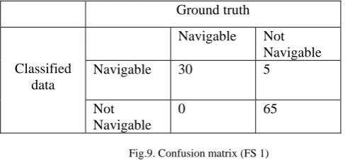
= (6) Confusion matrix of image (TI 1) is shown in fig. 9. It can be deduced from the table that correct classifIcation rate (classification accuracy) of the terrain classifier is 95% for this image as 95 sub terrainian regions which are navigable are correctly classified.
Ground truth
Classified data
Navigable Not
Navigable Navigable 30 5
Not Navigable
0 65
Fig.9. Confusion matrix (FS 1)
Confusion matrix using feature set 2 is shown in fig. 10 .It can be deduced from the matrix that the corect classification rate is 79%.Thus the correct rate using our feature set (FS 1) performed better than the other two feature sets.
Ground truth
Classified data
Navigable Not
Navigable Navigable 15 20 Not
Navigable
1 64
Fig.10 Confusion matrix (FS 2)
F i g . 1 1 s h o w s t h e c o n f u s i o n m a t r i x u s i n g f e a t u r e s e t 3 o n s a m e i m a g e ( T I 2 ) i n d i c a t i n g t h a t t h e c o r r e c t c l a s s i f i a c t i o n r a t e i s 8 5 %
Ground truth
Classified data
Navigable Not
Navigable Navigable 28 7
Not Navigable
7 58 Fig.11. Confusion matrix (FS 3)
The result obtained by using our approach gives an accuracy of 96 % as compared to feature set 1 which gives 93 % correct classification and feature set 2 giving only 94 % accuracy for the test image. Results on real time image captured from IIITDM campus also shows that our approach performs better than rest of the two feature sets.
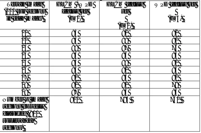
Table 1. Correct classification (%) for Mar’s terrain images
Terrain Image (100 sub regions
in each image)
GLCM +WPD feature set
(FS1)
GLCM feature set (FS2)
WPD feature set (FS3)
1 88 86 96
2 95 79 85
3 94 92 93
4 9 7 96 96
5 9 6 96 96
6 9 5 95 93
7 9 7 89 90
8 9 2 94 92
9 9 7 95 93
10 9 7 91 96
11 95 87 85
Number of image regions
correctly classified (1100
subterranean regions)
1043 904 1004
Table II. Correct classification (%) for real time terrain images of IIITDM campus
Terrain Image (100 sub regions
in each image)
GLCM +WPD feature set
(FS1)
GLCM feature set (FS2)
WPD feature set (FS3)
11 93 92 92
12 85 89 80
13 88 87 76
14 95 86 84
15 94 88 90
16 94 92 93
17 82 85 82
18 82 91 78
19 87 85 85
Number of image regions correctly classified (900 subterranean regions)
Fig.12. is the graph for correct classification rate for each of 20 images.
Fig.12. Graph showing correct classification rate
Mean success rate of the classifier using two feature sets is shown in fig. 13 for different image databases.
Fig.13. Graph of mean success rate
6. CONCLUSION AND FUTURE ASPECTS
In future, this line of inquiry can be continued to develop improved terrain classifier that will able to differentiate more than two classes (navigable or not navigable) and should identify sandy, rocky and muddy terrain in the not navigable region. Also, addition feature could be used to improve the classification accuracy. Further, the effects of employing different wavelets and alternative classifier architecture (such as support vector machines) to yield better classification accuracies on the terrain classification will also be investigated.
Another promising avenue would be to the hardware implementation of this intelligence on a real time robotic platform equipped with high precision vision sensors.
Acknowledgments
This work was supported by Indian Institute of Information Technology ,Design and Manufacturing Jabalpur MP India
REFERENCES
[1] Howard A., Tunstel E., Edwards D., "An Intelligent Terrain Based Navigation System for Planetary Rovers” in the Joint 9th IFSA World Congress and 20th NAFIPS Int. Conf., pp. 7-12, Vancouver, B.C.,Canada, July 2001
[2] Olson C. F., Matthies L. H., Wright J. R., "Visual Terrain Mapping for Mars Exploration," IEEE Aerospace Conference, paper #1176, 2003.
[3] Iagnemma K., A Brooks ,”Self-Supervised Classification for Planetary Rover Terrain Sensing” IEEE Aerospace Conference, March 2007
[4] Vandapel N., Huber, Kapuria D.F.,and Hebert,M. “Natural Terrain Classification using 3-D Ladar Data”. Proceedings of the 2003 IEEE International Conference on Robotics and Automation. Pp. 5117-5122
[5] Manduchi R.,. Castano, A., Talukder, A., and Matthies,L “Obstacle Detection and Terrain Classification for Autonomous Off-Road Navigation”. Autonomous Robots Vol. 18. Pp. 81-102
[6] Shirkhodaie A., Amrani R., and Chawla N., "Traversable Terrain Modeling and Performance Measurement of Mobile Robots,” Performance Metrics for Intelligent Systems Workshop, NIST, August 24-26, 2004
[7] Wolf D F., Dieter Fox and Burgard W., “Autonomous Terrain Classification Using Hidden Markov Models” Proceedings of the 2005 IEEE International Conference on Robotics and Automation [8]. A.Kelly, A., et al. (2006, June). “Toward Reliable Off Road Autonomous Vehicles Operating in Challenging Environments,” The International Journal of Robotics Research. 25(5/6).
[8] Dima C.S, Vandapel, N., and Hebert, M. (2004). “Classifier Fusion for outdoor obstacle detection,” Proceedings of the IEEE International Conference on Robotics and Automation (ICRA)1, 665-671, doi 10.1109/ROBOT.2004.1307225
[9] Birk A., Stoyanov Nevatia T, Y., ”Terrain Classification for Autonomous Robot Mobility :from Safety, Security Rescue Robotics to Planetory Explorations”, Proceedings of the IEEE International Conference on Robotics and Automation (ICRA), 2008
[10] Soennekar J, ”Machine Learning and Terrain Classification from LADAR Data”
[11] Poppinga J., A Birk and K. Pathak,”Hough Based Terrain Classification for real-time detection of derivable ground,” Journal of field Robotics, 2007
[12] Amrani R., "Visual Terrain Traversability Analysis and Assessment Based on Soft Computing Techniques," Master Thesis, Dept. of Mechanical and Manufacturing Engr., Tennessee State University, August 2004.
[13] Edmond. M. DuPont, Moore C.A and Jr. · Eric Coyle, “ Frequency Response method for Terrain Classification in Autonomous ground vehicle “, Journal of Field robotics ACMPotal,2008
[14] Mars Analyst’s Notebook 2006 fromhttp://anserverl.eprsl.wustl.edu/.
[15] Halatci I,,Christopher a.Brooks,” Terrain Classification and Classifier Fusion for Planetory Exploration Rovers,”IEEE Aerospace Conference (2007)