https://doi.org/10.5194/npg-25-429-2018 © Author(s) 2018. This work is distributed under the Creative Commons Attribution 4.0 License.
Sensitivity analysis with respect to observations in variational data
assimilation for parameter estimation
Victor Shutyaev1,2,3, Francois-Xavier Le Dimet4, and Eugene Parmuzin1,3
1Institute of Numerical Mathematics, Russian Academy of Sciences, Gubkina 8, Moscow 119333, Russia
2Federal State Budget Scientific Institution “Marine Hydrophysical Institute of RAS”, Kapitanskaya 2, Sevastopol 3Moscow Institute for Physics and Technology, 9 Institutskiy per., Dolgoprudny, Moscow Region, 141701, Russia 4LJK, Université Grenoble Alpes, 700 Avenue Centrale, 38401 Domaine Universitaire de Saint-Martin-d’Hères, Grenoble, France
Correspondence:Victor Shutyaev ([email protected]) Received: 22 January 2018 – Discussion started: 7 February 2018
Revised: 23 May 2018 – Accepted: 25 May 2018 – Published: 21 June 2018
Abstract.The problem of variational data assimilation for a nonlinear evolution model is formulated as an optimal con-trol problem to find unknown parameters of the model. The observation data, and hence the optimal solution, may con-tain uncercon-tainties. A response function is considered as a functional of the optimal solution after assimilation. Based on the second-order adjoint techniques, the sensitivity of the response function to the observation data is studied. The gra-dient of the response function is related to the solution of a nonstandard problem involving the coupled system of direct and adjoint equations. The nonstandard problem is studied, based on the Hessian of the original cost function. An algo-rithm to compute the gradient of the response function with respect to observations is presented. A numerical example is given for the variational data assimilation problem related to sea surface temperature for the Baltic Sea thermodynamics model.
1 Introduction
The methods of data assimilation have become an important tool for analysis of complex physical phenomena in vari-ous fields of science and technology. These methods allow us to combine mathematical models, data resulting from ob-servations, and a priori information. The problems of vari-ational data assimilation can be formulated as optimal con-trol problems (e.g., Lions, 1968; Le Dimet and Talagrand, 1986) to find unknown model parameters, such as initial
and/or boundary conditions, right-hand sides in the model equations (forcing terms), and distributed coefficients, based on minimization of the cost function related to observations. A necessary optimality condition reduces an optimal control problem to an optimality system which involves the model equations, the adjoint problem, and input data functions. The optimal solution depends on the observation data, and for fu-ture forecasts it is very important to study the sensitivity of the optimal solution with respect to observation errors (Baker and Daley, 2000).
The necessary optimality condition is related to the gradi-ent of the original cost function; thus, to study the sensitivity of the optimal solution, one should differentiate the optimal-ity system with respect to observations. In this case, we come to the so-called second-order adjoint problem (Le Dimet et al., 2002). The first studies of sensitivity of the response func-tions after assimilation with the use of second-order adjoint were done by Le Dimet et al. (1997) for variational data as-similation problems aimed at restoration of initial condition, where sensitivity with respect to model parameters was con-sidered. The equations of the forecast sensitivity to observa-tions in a four-dimensional (4D-Var) data assimilation were derived by Daescu (2008). Based on these results, a practical computational approach was given by Cioaca et al. (2013) to quantify the effect of observations in 4D-Var data assimila-tion.
variational data assimilation with respect to observations for a nonlinear dynamic model was given by Shutyaev et al. (2017) to control the initial-value function. The dynamic for-mulation of the problem is important because it shows differ-ent implemdiffer-entation options (Gejadze et al., 2018).
This paper is based on the results of Shutyaev et al. (2017) and presents the sensitivity analysis with respect to observa-tions in variational data assimilation aimed at restoration of unknown parameters of a dynamic model. We should men-tion the importance of the parameter estimamen-tion problem it-self. A precise determination of the initial condition is very important in view of forecasting; however, the use of vari-ational data assimilation is not limited to opervari-ational fore-casting. In many domains (e.g., hydrology) the uncertainty in the parameters is more crucial than the uncertainty in the initial condition (e.g., White at al., 2003). In some problems the quantity of interest can be represented directly by the es-timated parameters as controls. For example, in Agoshkov et al. (2015) the sea surface heat flux is estimated in order to un-derstand its spatial and temporal variability. The problems of parameter estimation are common inverse problems consid-ered in geophysics and in engineering applications (see Ali-fanov et al., 1996; Sun, 1994; Zhu and Navon, 1999; Storch et al., 2007). In the last years, interest in the parameter esti-mation using 4D-Var is rising (Bocquet, 2012; Schirber at al., 2013; Yuepeng et al., 2018; Agoshkov and Sheloput, 2017).
We consider a dynamic formulation of the variational data assimilation problem for parameter estimation in a continu-ous form, but the presented sensitivity analysis formulas with respect to observations do not follow from our previous re-sults for the initial condition problem (Shutyaev et al., 2017) and constitute a novelty of this paper. Of course, the initial condition function may also be considered as a parameter; however, in our dynamic formulation we have two equations for the model: one equation for describing an evolution of the model operator (involving model parameters such as right-hand sides, coefficients, boundary conditions, etc.) and an-other equation is considered as an initial condition.
This paper is organized as follows. In Sect. 2, we give the statement of the variational data assimilation problem for a nonlinear evolution model to estimate the model parameters. In Sect. 3, sensitivity of the response function after assimi-lation with respect to observations is studied, and its gradi-ent is related to the solution of a nonstandard problem. In Sect. 4 we derive an operator equation involving the Hes-sian to study the solvability of the nonstandard problem, and give an algorithm to compute the gradient of the response function. A proof-of-concept analytic example with a simple model is given in Sect. 5 to demonstrate how the sensitivity analysis algorithm works. Section 6 presents an application of the theory to the data assimilation problem for a sea ther-modynamics model. Numerical examples are given in Sect. 7 for the Baltic Sea dynamics model. The main results are dis-cussed in Sect. 8.
2 Statement of the problem
We consider the mathematical model of a physical process that is described by the evolution problem
∂ϕ
∂t =F (ϕ, λ)+f, t∈(0, T ) ϕ
t=0 =u,
(1)
where the initial stateu belongs to a Hilbert spaceX,ϕ=
ϕ(t )is the unknown function belonging toY=L2(0, T;X) with the normkϕkY =(ϕ, ϕ)Y1/2=(R0Tkϕ(t )k2
Xdt )1/2,F is
a nonlinear operator mappingY×YpintoY,Ypis a Hilbert space (space of control parameters, or control space), and f ∈Y. Suppose that for a givenu∈X, f ∈Y, andλ∈Yp, there exists a unique solutionϕ∈Y to Eq. (1) with ∂ϕ∂t ∈Y. The functionλis an unknown model parameter. Let us intro-duce the cost function
J (λ)=1
2(V1(λ−λb), λ−λb)Yp (2)
+1
2(V2(Cϕ−ϕobs), Cϕ−ϕobs)Yobs,
whereλb∈Ypis a prior (background) function,ϕobs∈Yobs is a prescribed function (observational data),Yobsis a Hilbert space (observation space),C:Y→Yobsis a linear bounded observation operator, andV1:Yp→YpandV2:Yobs→Yobs are symmetric positive definite bounded operators.
Let us consider the following data assimilation problem with the aim to estimate the parameter λ: for a given u∈
X,andf ∈Y, findλ∈Ypandϕ∈Y such that they satisfy Eq. (1), and on the set of solutions to Eq. (1), the functional J (λ)takes the minimum value, i.e.,
∂ϕ
∂t =F (ϕ, λ)+f, t∈(0, T ) ϕ
t=0 =u, J (λ) = inf
v∈Yp
J (v).
(3)
We suppose that the solution of Eq. (3) exists. Let us note that the solvability of the parameter estimation problems (or identifiability) has been addressed, e.g., in Chavent (1983) and Navon (1998). To derive the optimality system, we as-sume the solutionϕand the operatorF (ϕ, λ)in Eqs. (1)–(2) are regular enough, and forv∈Yp find the gradient of the functionalJ with respect toλ:
J0(λ)v=(V1(λ−λb), v)Yp+(V2(Cϕ−ϕobs), Cφ)Yobs (4)
=(V1(λ−λb), v)Yp+(C
∗
V2(Cϕ−ϕobs), φ)Y,
whereφis the solution to the problem:
∂φ
∂t = F 0
ϕ(ϕ, λ)φ+F
0
λ(ϕ, λ)v,
φ
t=0 = 0.
Here Fϕ0(ϕ, λ):Y→Y, Fλ0(ϕ, λ):Yp→Y are the Fréchet derivatives ofF (Marchuk et al., 1996) with respect toϕand λ, correspondingly, andC∗is the adjoint operator toC de-fined by(Cϕ, ψ )Yobs=(ϕ, C
∗ψ )
Y, ϕ∈Y, ψ∈Yobs. Let us consider the adjoint operator(Fϕ0(ϕ, λ))∗:Y →Y and introduce the adjoint problem:
∂ϕ∗ ∂t +(F
0
ϕ(ϕ, λ))
∗ϕ∗ = C∗V
2(Cϕ−ϕobs),
ϕ∗t=T = 0.
(6)
Then Eq. (4) with Eqs. (5) and (6) gives J0(λ)v=(V1(λ−λb), v)Yp−(ϕ
∗
, Fλ0(ϕ, λ)v)Y (7) =(V1(λ−λb), v)Yp−((F
0
λ(ϕ, λ))
∗ϕ∗, v)
Yp,
where (Fλ0(ϕ, λ))∗:Y →Yp is the adjoint operator to Fλ0(ϕ, λ). Therefore, the gradient ofJis defined by
J0(λ)=V1(λ−λb)−(Fλ0(ϕ, λ))∗ϕ∗.
From Eqs. (4)–(7) we get the optimality system (the nec-essary optimality conditions; Lions, 1968):
∂ϕ
∂t =F (ϕ, λ)+f, t∈(0, T ), ϕt=0 =u,
(8)
∂ϕ∗ ∂t +(F
0
ϕ(ϕ, λ))
∗
ϕ∗ = C∗V2(Cϕ−ϕobs), ϕ∗
t=T = 0,
(9)
V1(λ−λb)−(Fλ0(ϕ, λ))∗ϕ∗=0. (10) We assume that the system (Eqs. 8–10) has a unique solu-tion. The system (Eqs. 8–10) may be considered as a general-ized modelA(U )=0 with the state variableU=(ϕ, ϕ∗, λ), and it contains information about observations. In what fol-lows we study the problem of the sensitivity of functionals of the optimal solution to the observation data.
If the observation operator C is nonlinear, i.e., Cϕ=
C(ϕ), then the right-hand side of the adjoint equation (Eq. 9) contains(Cϕ0)∗ instead ofC∗ and all the analysis presented below is similar.
3 Sensitivity of functionals after assimilation
In geophysical applications the observation data cannot be measured precisely; therefore, it is important to be able to estimate the impact of uncertainties in observations on the outputs of the model after assimilation.
Let us introduce a response function G(ϕ, λ), which is supposed to be a real-valued function and can be considered as a functional onY×Yp. We are interested in the sensitivity
ofG with respect toϕobs, withϕ andλ obtained from the optimality system (Eqs. 8–10). By definition, the sensitivity is defined by the gradient ofGwith respect toϕobs:
dG dϕobs
=∂G
∂ϕ ∂ϕ ∂ϕobs
+∂G
∂λ ∂λ ∂ϕobs
. (11)
Ifδϕobsis a perturbation onϕobs, we get from the optimal-ity system:
∂δϕ
∂t = F 0
ϕ(ϕ, λ)δϕ+Fλ0(ϕ, λ)δλ,
δϕ
t=0 = 0,
(12)
−∂δϕ
∗ ∂t −(F
0
ϕ(ϕ, λ))
∗δϕ∗−(F00
ϕϕ(ϕ, λ)δϕ)
∗ϕ∗
=(Fϕλ00 (ϕ, λ)δλ)∗ϕ∗−C∗V2(Cδϕ−δϕobs),
δϕ∗
t=T =0,
(13)
V1δλ−(Fλϕ00 (ϕ, λ)δϕ)
∗
ϕ∗−(Fλλ00(ϕ, λ)δλ)∗ϕ∗ (14)
−(Fλ0(ϕ, λ))∗δϕ∗=0, and
dG
dϕobs, δϕobs
Yobs
=
∂G ∂ϕ, δϕ
Y +
∂G ∂λ, δλ
Yp
, (15)
whereδϕ,δϕ∗, andδλare the Gâteaux derivatives ofϕ,ϕ∗, andλin the directionδϕobs(for example,δϕ= ∂ϕ
∂ϕobsδϕobs).
To compute the gradient ∇ϕ
obsG(ϕ, λ), let us introduce
three adjoint variablesP1∈Y,P2∈Y, andP3∈Yp. By tak-ing the inner product of Eq. (12) byP1, Eq. (13) byP2, and of Eq. (14) byP3and adding them,
∂δϕ
∂t −F 0
ϕ(ϕ, λ)δϕ−F
0
λ(ϕ, λ)δλ, P1
Y
+
−∂δϕ
∗ ∂t −(F
0
ϕ(ϕ, λ))
∗
δϕ∗−(Fϕϕ00 (ϕ, λ)δϕ)∗ϕ∗
−(Fϕλ00 (ϕ, λ)δλ)∗ϕ∗+C∗V2(Cδϕ−δϕobs), P2
Y
+
V1δλ−(Fλϕ00 (ϕ, λ)δϕ)∗ϕ∗−(Fλλ00(ϕ, λ)δλ)∗ϕ∗
−(Fλ0(ϕ, λ))∗δϕ∗, P3
Yp=0.
δϕ,−∂P1
∂t −(F 0
ϕ(ϕ, λ))
∗
P1−(Fϕϕ00 (ϕ, λ)P2)∗ϕ∗
−(Fλϕ00 (ϕ, λ)P3)∗ϕ∗+C∗V2CP2
Y
+ δϕ t=T, P1
t=T
X
+
δϕ∗,∂P2 ∂t −F
0
ϕ(ϕ, λ)P2−Fλ0(ϕ, λ)P3
Y
+ δϕ∗ t=0, P2
t=0
X+
δλ, V1P3−(Fϕλ00(ϕ, λ)P2)∗ϕ∗
−(Fλλ00(ϕ, λ)P3)∗ϕ∗−(Fλ0(ϕ, λ))∗P1Y
p
−(δϕobs, V2CP2)Yobs=0. (16) Here we put
−∂P1
∂t −(F 0
ϕ(ϕ, λ))
∗
P1−(Fϕϕ00 (ϕ, λ)P2)∗ϕ∗
−(Fλϕ00 (ϕ, λ)P3)∗ϕ∗+C∗V2CP2= ∂G
∂ϕ,
and
V1P3−(Fϕλ00(ϕ, λ)P2)∗ϕ∗−(Fλλ00(ϕ, λ)P3)∗ϕ∗
−(Fλ0(ϕ, λ))∗P1=∂G
∂λ, P1
t=,T =0,
∂P2 ∂t −F
0
ϕ(ϕ, λ)P2−Fλ0(ϕ, λ)P3=0, P2
t=0=0.
Thus, if P1, P2, and P3 are the solutions of the following system of equations
−∂P1
∂t −(F 0
ϕ(ϕ, λ))
∗
P1−(Fϕϕ00 (ϕ, λ)P2)∗ϕ∗
=(Fλϕ00 (ϕ, λ)P3)∗ϕ∗−C∗V2CP2+ ∂G
∂ϕ, P1
t=T =0,
(17)
∂P2 ∂t −F
0
ϕ(ϕ, λ)P2−Fλ0(ϕ, λ)P3 = 0, t∈(0, T ) P2
t=0 = 0,
(18) V1P3−(Fϕλ00(ϕ, λ)P2)∗ϕ∗−(Fλλ00(ϕ, λ)P3)∗ϕ∗ (19)
−(Fλ0(ϕ, λ))∗P1= ∂G
∂λ, then from Eq. (16) we get
∂G ∂ϕ, δϕ Y + ∂G ∂λ, δλ Yp
=(δϕobs, V2CP2)Yobs,
and due to Eq. (15) the gradient ofGis given by dG
dϕobs
=V2CP2. (20)
We get a coupled system of two differential equations (Eqs. 17 and 18) of the first order with respect to time, and Eq. (19). To study this nonstandard problem (Eqs. 17–19), we reduce it to a single operator equation involving the Hes-sian of the original cost function.
4 Operator equation via Hessian and response function gradient
Let us denote the auxiliary variablev=P3and rewrite the nonstandard problem (Eqs. 17–19) in an equivalent form:
∂P2 ∂t −F
0
ϕ(ϕ, λ)P2 = Fλ0(ϕ, λ)v,
P2
t=0 = 0,
(21)
−∂P1
∂t −(F 0
ϕ(ϕ, λ))
∗
P1−(Fϕϕ00 (ϕ, λ)P2)∗ϕ∗
=(Fλϕ00 (ϕ, λ)v)∗ϕ∗−C∗V2CP2+ ∂G
∂ϕ, P1
t=T =0,
(22)
V1v−(Fϕλ00 (ϕ, λ)P2)∗ϕ∗−(Fλλ00(ϕ, λ)v)
∗
ϕ∗ (23)
−(Fλ0(ϕ, λ))∗P1=∂G
∂λ.
Here we have three unknowns:v∈Yp, P1, andP2∈Y. Let us write Eqs. (21)–(23) in the form of an operator equation forv. We define the operatorH, which acts onwbelonging toYp, by the successive solution of the following problems:
∂φ ∂t −F
0
ϕ(ϕ, λ)φ = Fλ0(ϕ, λ)w, t∈(0, T )
φ
t=0 = 0,
(24) −∂φ ∗ ∂t −(F
0
ϕ(ϕ, λ))
∗
φ∗−(Fϕϕ00 (ϕ, λ)φ)∗ϕ∗
=(Fλϕ00 (ϕ, λ)w)∗ϕ∗−C∗V2Cφ, φ∗t=T =0,
(25)
Hw=V1w−(Fϕλ00(ϕ, λ)φ)∗ϕ∗ (26)
−(Fλλ00(ϕ, λ)w)∗ϕ∗−(Fλ0(ϕ, λ))∗φ∗.
Hereλ, ϕ, andϕ∗are the solutions of the optimality system (Eqs. 8–10). Then Eqs. (21)–(23) are equivalent to the fol-lowing equation inYp:
Hv=F (27)
with the right-hand sideFdefined by F=∂G
∂λ +(F 0
λ(ϕ, λ))
∗
e
φ∗, (28)
whereeφ∗is the solution to the adjoint problem:
−∂φe
∗ ∂t −(F
0
ϕ(ϕ, λ))
∗
e
φ∗ = ∂G
∂ϕ, t∈(0, T )
e
φ∗
t=T = 0.
It is easily seen that the operatorHdefined by Eqs. (24)– (26) is the Hessian of the original functionalJconsidered on the optimal solutionλof the problem (Eqs. 8–10):J00(λ)= H. Under the assumption thatHis positive definite, the op-erator equation (Eq. 27) is correctly and everywhere solvable inYp(Vainberg, 1964), i.e., for everyFthere exists a unique solutionv∈Ypand
kvkY
p≤ckFkYp, c=const>0.
Therefore, under the assumption thatJ00(λ)is positive def-inite on the optimal solution, the nonstandard problem (Eqs. 17–19) has a unique solutionP1, P2∈Y, andP3∈Yp. Based on the above consideration, we can formulate the following algorithm to compute the gradient of the response functionG:
1. For∂G∂λ ∈Yp, and ∂G∂ϕ ∈Y solve the adjoint problem
−∂eφ
∗ ∂t −(F
0
ϕ(ϕ, λ))
∗
e
φ∗ = ∂G
∂ϕ,
e
φ∗
t=T = 0
(30)
and put F=∂G
∂λ +(F 0
λ(ϕ, λ))
∗
e
φ∗.
2. Findvby solving Hv=F
with the Hessian of the original functionalJdefined by Eqs. (24)–(26).
3. Solve the direct problem
∂P2 ∂t −F
0
ϕ(ϕ, λ)P2 = Fλ0(ϕ, λ)v, t∈(0, T )
P2
t=0 = 0.
(31) 4. Compute the gradient of the response function as
dG dϕobs
=V2CP2. (32)
Equation (32) allows us to estimate the sensitivity of the functionals related to the optimal solution after assimilation, with respect to observation data.
Remark 1. In the above consideration, to show the
solv-ability, we have assumed that the direct and adjoint tangent linear problems of the form
∂φ ∂t −F
0
ϕ(ϕ, λ)φ = f, t∈(0, T )
φ
t=0 = 0,
−∂φ
∗ ∂t −(F
0
ϕ(ϕ, λ))
∗φ∗ = g, t∈(0, T ) φ∗t=T = 0
withf, g∈Y have the unique solutionsφ, φ∗∈Y.
Remark 2.The analysis presented above is based on the
hypothesis that the initial state of the system under observa-tion is known, and that it is only model parameters (boundary conditions, forcing terms, distributed coefficients, etc.) that are to be determined from the observations. Often, a more realistic situation would be one where the assimilation is in-tended to determine both the initial conditions of the system and, in addition, model parameters (Dee, 2005; Smith et al., 2013). The sensitivity analysis can be applied as well to such a situation. To consider the joint state and parameter estima-tion problem, we should use the results both of this paper and of the previous one (Shutyaev et al., 2017). In this case we need to introduce an additional term related to the initial condition into the cost function (Eq. 2) to find simultaneously uandλ. The optimality system (Eqs. 8–10) will be supple-mented by an additional equation related to the gradient of the cost function with respect tou. The Hessian in this case is a 2×2 operator matrix, acting on the augmented vector U=(u, λ)T, and all the derivations are made similarly, be-ing, however, more cumbersome and lengthy.
Below we give a proof-of-concept analytic example to show how the algorithm (Eqs. 30–32) works. Then, as an ap-plication, we consider a variational data assimilation problem for a sea thermodynamics model.
5 Proof-of-concept analytic example
Let us consider a simple evolution problem for the ordinary differential equation
dϕ
dt +aϕ = λg, t∈(0, T ) ϕ
t=0 = u,
(33)
whereu∈R;a, λ∈R;g=g(t )≥0. Here, in the notations of Sect. 2, we have X=R, Y =L2(0, T ), andF (ϕ, λ)= −aϕ+λg. Let us formulate the data assimilation problem to find the parameterλif we have observation data forϕat the end of the time intervalt=T. We need to minimize the cost function
J (λ)= inf
v∈RJ (v), (34)
where J (v)=1
2
eϕ|t=T−ϕobs
2
(Eqs. 8–10) has the form:
dϕ
dt +aϕ=λg, t∈(0, T ) ϕ
t=0=u,
(35)
dϕ∗ dt −aϕ
∗=
0, t∈(0, T ) ϕ∗
t=T =ϕ
t=T −ϕobs,
(36)
(g, ϕ∗)= T Z
0
g(t )ϕ∗(t )=0. (37)
It is easy to see that the problem of data assimilation (Eqs. 33–34) has a unique solution
λ=λopt=ϕobs−ϕ0
ϕ1 , (38)
whereϕ0=u0e−aT,ϕ1= T R
0
e−a(T−t0)g(t0)dt0.
Indeed, if λ has the form (Eq. 38), the solution of the problem (Eq. 33) satisfies ϕ|t=T =ϕobs, and the functional J from Eq. (34) attains its minimal valueJ=0. In this case ϕ∗=0, and the optimality system (Eqs. 35–37) is satisfied. Let us consider the response function in the form
G (ϕ, λ)= T Z
0
ϕ(t )dt. (39)
Leta6=0. After assimilation, taking into account the solu-tion of the problem (Eq. 33), we have
G(ϕ, λ)=u
a
1−e−aT+λopt
a
T Z
0
g(t )dt−ϕ1
, (40)
whereλoptis given by Eq. (38). Then, by differentiation of Gwith respect toϕobswe have the gradient
dG dϕobs =
1 aϕ1
T Z
0
g(t )dt−ϕ1
. (41)
Let us now apply the algorithm (Eqs. 30–32) to com-pute the gradient of the function G. Since ∂G∂ϕ =1, and (Fϕ0(ϕ, λ))∗= −a, then on the first step of the algorithm, we solve the problem (Eq. 30) and get the solution
e
φ∗(t )= 1
a
1−e−a(T−t ). (42)
Taking into account that∂G/∂λ=0 and (Fϕ0(ϕ, λ))∗eφ∗=
(g,eφ
∗), we getF=(g,
e
φ∗), i.e.,
F= T Z
0
gφe∗dt=
1 a
T Z
0
g(t )dt−ϕ1
. (43)
On the second step of the algorithm, one needs to solve the equationHv=Fwith the HessianHdefined by Eqs. (24)– (26). Since all the second-order derivatives ofF (ϕ, λ)equal zero, then it is easily seen thatHin this case is the operator of multiplication by the scalar
H=
T Z
0
g(t )ψ|t=Te−a(T−t )dt=(ψ|t=T)2, (44)
whereψ (t )is the solution of the problem (Eq. 33) withu=
0, andλ=1. Then, after the second step of the algorithm we get
v=H−1F=(ψ|t=T)−2F. (45) On the third step of the algorithm, we need to solve the problem (Eq. 31). SinceFλ0(ϕ, λ)=g, the solution of this problem has the formP2(t )=vψ (t ). Finally, using Eq. (32), we get the gradient ofGwith respect toϕobs:
dG dϕobs
=P2|t=T =vψ (T )=
ψ (T )F ψ2(T ) =
F
ψ (T ). (46) Moreover, sinceϕ1=ψ (T ), then from Eqs. (46) and (43) we have
dG dϕobs
= 1
aϕ1
T Z
0
g(t )dt−ϕ1
. (47)
Thus, the gradient obtained by the algorithm (Eqs. 30–32) exactly coincides with the value of the gradient obtained in Eq. (41) by direct differentiation, which is the expected re-sult.
6 Data assimilation problem for a sea thermodynamics model
Consider the sea thermodynamics problem in the form (Marchuk et al., 1987):
Tt+(U ,Grad)T−Div(aˆT·GradT )=fT inD×(t0, t1),
T =T0fort=t0inD,
−νT
∂T
∂z =Qon0S×(t0, t1), ∂T
∂n =0 on0w,c×(t0, t1), U(n−)T+∂T
∂n =QT on0w,op×(t0, t1), ∂T
where T =T (x, y, z, t ) is an unknown temperature func-tion, t∈(t0, t1), (x, y, z)∈D=×(0, H ), ⊂R2, H=
H (x, y)is the function of the bottom relief,Q=Q(x, y, t ) is the total heat flux, U=(u, v, w), baT =diag((aT)ii),
(aT)11=(aT)22=µT,(aT)33=νT, andfT =fT(x, y, z, t )
are given functions. The boundary of the domain0≡∂Dis represented as a union of four disjoint parts0S,0w,op,0w,c, and0H, where0S=(the unperturbed sea surface),0w,op is the liquid (open) part of vertical lateral boundary,0w,cis the solid part of the vertical lateral boundary, 0H is the sea bottom,U(n−)=(|Un| −Un)/2,andUnis the normal com-ponent ofU. The other notations and a detailed description of the problem statement can be found in Agoshkov et al. (2008).
Equation (48) can be written in the form of an operator equation:
Tt+LT =F+BQ, t∈(t0, t1),
T =T0, t=t0, (49)
where the equality is understood in the weak sense, namely, (Tt,bT )+(LT ,T )b =F(T )b +(BQ,T )b ∀Tb∈W21(D), (50)
in this caseL,F, and B are defined by the following rela-tions:
(LT ,T )b ≡ Z
D
(−TDiv(UT ))dDb + Z
0w,op
U(n+)TTbd0
+ Z
D
baTGrad(T )·Grad(T )dD,b
F(T )b = Z
0w,op
QTbTd0+ Z
D
fTbTdD, (Tt,T )b = Z
D
TtbTdD,
(BQ,bT )= Z
QbT
z=0d,
and the functionsbaT,QT,fT, andQare such that Eq. (50)
makes sense. The properties of the operatorLwere studied by Agoshkov et al. (2008).
Due to Eq. (50), Eq. (49) is considered in Y∗=L2(t0, t1;(W21(D))∗), and the operator B:L2(× (t0, t1))→Y∗ maps the function Q∈L2(×(t0, t1)) into the function BQ∈Y∗ such that (BQ,bT )=
R
QTb
z=0d,
∀bT ∈W21(D). Therefore, BQ is a linear and bounded functional onL2(0, T;W21(D)).
Consider the data assimilation problem for the sea surface temperature (see Agoshkov et al., 2008). Suppose that the function Q∈L2(×(t0, t1)) is unknown in Eq. (48). Let Tobs(x, y, t )also be the function on≡∪∂obtained for t∈(t0, t1)by processing the observation data, and this func-tion in its physical sense is an approximafunc-tion to the surface
temperature function on, i.e., toT
z=0. We suppose that Tobs∈L2(×(t0, t1)), but the function Tobs may not pos-sess greater smoothness and hence it cannot be used for the boundary condition on0S. We admit the case whenTobsis defined only on some subset of×(t0, t1)and denote the indicator (characteristic) function of this set bym0. For defi-niteness sake, we assume thatTobsis zero outside this subset. Consider the data assimilation problem for the surface temperature in the following form: findT andQsuch that
Tt+LT = F+BQinD×(t0, t1), T = T0, t=t0
J (Q) = inf
vJ (v),
(51)
where
J (Q)=α
2
t1
Z
t0
Z
|Q−Q(0)|2ddt
+1
2
t1
Z
t0
Z
m0|T
z=0−Tobs|
2ddt, (52)
andQ(0)=Q(0)(x, y, t )is a given function, andα=const> 0.
Forα >0 this variational data assimilation problem has a unique solution. The existence of the optimal solution fol-lows from the classic results of the theory of optimal con-trol problems (Lions, 1968), because it is easy to show that the solution to Eq. (48) continuously depends on the fluxQ (a priori estimates are valid in the corresponding functional spaces), the functionalJ is weakly lower semi-continuous, and the space of admissible controls L2(×(t0, t1)) is weakly compact.
Forα=0 the problem does not always have a solution, but, as was shown by Agoshkov et al. (2008), there is unique and dense solvability, and it allows one to construct a se-quence of regularized solutions minimizing the functional, which is related to a sequence of coefficientsαn, withαn→0
whenn→ ∞.
The optimality system determining the solution of the for-mulated variational data assimilation problem according to the necessary condition gradJ=0 has the form:
Tt+LT =F+BQin D×(t0, t1), (53)
T =T0, t=t0,
−(T∗)t+L∗T∗=Bm0(Tobs−T )inD×(t0, t1), (54)
T∗=0, t=t1,
α(Q−Q(0))−T∗=0 on×(t0, t1), (55) whereL∗is the operator adjoint toL.
−LT +BQ, and FT0 = −L, FQ0 =B. Since the operator F (T , Q) is bilinear in this case, the HessianH acting on some ψ∈L2(×(t0, t1)) is defined by the successive so-lution of the following problems:
∂φ
∂t +Lφ = Bψ, t∈(t0, t1) φt=t
0
= 0,
(56)
−∂φ
∗ ∂t +L
∗
φ∗ = −Bm0φ, t∈(t0, t1) φ∗t=t
1
= 0,
(57)
Hψ=αψ−B∗φ∗. (58)
To illustrate the above-presented theory, we consider the problem of sensitivity of functionals of the optimal solution Q to the observationsTobs. Let us introduce the following functional (response function):
G(T )= t1
Z
t0
dt
Z
k(x, y, t )T (x, y,0, t )d, (59)
wherek(x, y, t ) is a weight function related to the temper-ature field on the sea surface z=0. For example, if we are interested in the mean temperature of a specific region of the seaωforz=0 in the intervalt−τ ≤t≤t, then askwe take the function
k(x, y, t )=
1(τmesω) if(x, y)∈ω, t−τ ≤t≤t
0 else,
(60) where mesωdenotes the area of the regionω. Thus, Eq. (59) is written in the form:
G(T )=1
τ
t Z
t−τ
dt
1 mesω
Z
ω
T (x, y,0, t )d
. (61)
Equation (61) represents the mean temperature averaged over the time intervalt−τ ≤t≤tfor a given regionω. The functionals of this type are of most interest in the theory of climate change (Marchuk, 1995; Marchuk et al., 1996).
In our notations, Eq. (59) may be written as
G(T )= t1
Z
t0
(Bk, T )dt=(Bk, T )Y, Y =L2(D×(t0, t1)).
We are interested in the sensitivity of the functionalG(T ), obtained forT after data assimilation, with respect to the ob-servation functionTobs.
By definition, the sensitivity is given by the gradient ofG with respect toTobs:
dG dTobs
=∂G
∂T ∂T ∂Tobs
. (62)
Since∂G∂T =Bk, then, according to the theory presented in Sect. 4, to compute the gradient (Eq. 62) we need to perform the following steps:
1. Forkdefined by Eq. (60) solve the adjoint problem
−∂eφ
∗ ∂t +L
∗
e
φ∗ = Bk, t∈(t0, t1)
e
φ∗t=t
1
= 0
(63)
and put8=B∗eφ∗.
2. Findχby solvingHχ=8with the Hessian defined by Eqs. (56)–(58).
3. Solve the direct problem
∂P2
∂t +LP2 = Bχ , t∈(t0, t1) P2
t=t0 = 0.
(64)
4. Compute the gradient of the response function as dG
dTobs =m0P2
z=0. (65)
Equation (65) allows us to estimate the sensitivity of the functionals related to the mean temperature after data assim-ilation, with respect to the observations on the sea surface.
7 Numerical example for the Baltic Sea dynamics model
The numerical experiments have been performed using the three-dimensional numerical model of the Baltic Sea hydro-thermodynamics developed at the Institute of Numerical Mathematics, Russian Academy of Sciences on the base of the splitting method (Zalesny et al., 2017) and supplied with the assimilation procedure (Agoshkov et al., 2008) for the surface temperatureTobswith the aim to reconstruct the heat fluxesQ.
conditions and ran with atmospheric forcing obtained from reanalysis of about 20 years, and after that the result of cal-culation was taken as an initial condition for further running of the model. The assimilation procedure worked only dur-ing some time windows. To start the assimilation procedure for the heat flux estimation, the initial condition was taken as a model forecast for the previous time interval.
The Baltic Sea daily-averaged nighttime surface-temperature data were used for Tobs. These are the data of the Danish Meteorological Institute based on measure-ments of radiometers (AVHRR, AATSR, and AMSRE) and spectroradiometers (SEVIRI and MODIS) (Karagali, 2012). Data interpolation algorithms were used (Zakharova et al., 2013) to convert observations on computational grid of the numerical model of the Baltic Sea thermodynamics. For each time step the heat flux was determined at each surface point; therefore, the number of scalar parameters to be determined were equal to the number of scalar observations. The mean climatic flux obtained from the NCEP (National Centers for Environmental Prediction) reanalysis was taken forQ(0).We need to mention thatQ(0)has a physical mean-ing here, it is not only an initial guess but also a parameter calculated from atmospheric data and taken in the model for temperature boundary condition on the sea surface when the model runs without the assimilation procedure.
Using the hydro-thermodynamics model mentioned above, which is supplied with the assimilation procedure for the surface temperature Tobs, we have performed calcula-tions for the Baltic Sea area where the assimilation algo-rithm worked only at certain time moments t0; in this case t1=t0+1t.
The aim of the experiment was the numerical study of the sensitivity of functionals of the optimal solutionQto obser-vation errors in the interval(t0, t1).
Implementing the assimilation procedure, we considered a system of the form in Eqs. (53)–(55), where Eqs. (53)–(54) mean the finite-dimensional analogues of the corresponding problems (Agoshkov et al., 2008). For the statement of a data assimilation problem we introduce the cost function (Eq. 52) with a regularization parameterα, which weights the squared difference |Q−Q(0)|2. Since in all numerical experiments αwas chosen very small, the impact of the first term in the functional was also small, and thereforeQwas different from Q(0).
We use here the SI units, namely K (kelvin) is used for temperature, m s−1 for velocities, and mK s−1 for the heat flux Q. The parameterα is defined as s2m−2 to give both terms in Eq. (52) the same dimension. It is easily seen that in this case the units of the gradient ddTG
obs from Eq. (65) are
defined as m−2s−1.
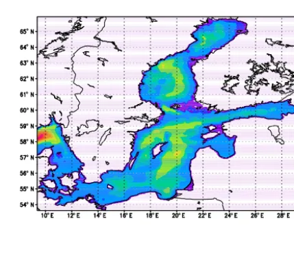
Let us present some results of numerical experiments. The calculation results fort0=50 h (600 time steps for the model) are presented in Fig. 1 showing the gradient of the functionalG(T )defined by Eq. (61) and related to the mean
Figure 1.The gradient of the functionalG(T )(m−2s−1).
Figure 2.Baltic Sea topography (m).
temperature after data assimilation, with respect to the obser-vations on the sea surface, according to Eqs. (63)–(65). Here ω=,τ =1t,t=t1, andα=10−5s2m−2.
We can see the sub-areas (in red) in which the functional G(T )is most sensitive to errors in the observations during assimilation. The largest values of the gradient ofG(T ) cor-respond to the pointsx, ylying near the regions with a small depth (cf. sea topography, Fig. 2). One explanation of this phenomenon may be the fact that in the areas with depths of about 50 m, rapid convection occurs in the upper mixed layer. With the assimilation of the surface temperature, in-formation is transmitted faster to shallower depths, which in turn contributes to a higher sensitivity to data in these places, in contrast to deeper regions.
Remark 3.We use the discretize-then-optimize approach,
are understood in a discrete form, as finite-dimensional ana-logues of the corresponding problems, obtained after approx-imation. This allows us to consider model equations as a per-fect model, with no approximation errors. Therefore, the ac-curacy of the sensitivity estimates given by Eqs. (63)–(65) are determined by the accuracy of solving the Hessian equa-tion Hχ=8(step 2 of the algorithm). Due to Eqs. (56)– (58), this equation is equivalent to a linear data assimilation problem, and an approximate solution to the minimization problem is obtained by an iterative procedure.
The above studies allow us to solve the problem of the def-inition of sea sub-areas in which the functional of the optimal solution is most sensitive to errors in the observations during variational data assimilation, when the error values are not a priori known.
8 Conclusions
In this paper we have considered numerical algorithms to study the sensitivity of functionals of the optimal solution of the variational data assimilation problem aimed at the re-construction of unknown parameters of the model. The op-timal solution obtained as a result of assimilation depends on the observations that may contain uncertainties. Comput-ing the gradient of the functionals with respect to observa-tions reduces to the solution of a nonstandard problem which is a coupled system involving direct and adjoint equations with mutually dependent variables. Solvability of the non-standard problem is related to the properties of the Hessian of the original cost function. An algorithm developed to com-pute the gradient of the response function is based on the second-order adjoint techniques. A numerical example for the variational data assimilation problem related to sea sur-face temperature for the Baltic Sea thermodynamics model demonstrates the result of the gradient computation of the response function associated with the mean surface tempera-ture. The presented algorithm may be used to determine the sea sub-areas in which the functionals of the optimal solu-tion are most sensitive to errors in the observasolu-tions during variational data assimilation.
Data availability. The Baltic Sea daily-averaged
surface-temperature data (Copernicus product ID
ST_BAL_SST_L4_REP_OBSERVATIONS_010_016) can be
found at the Copernicus Marine Environment Monitoring Ser-vice website (http://marine.copernicus.eu/services-portfolio/ access-to-products/).
Competing interests. The authors declare that they have no conflict
of interest.
Special issue statement. This article is part of the special
is-sue “Numerical modeling, predictability and data assimilation in weather, ocean and climate: A special issue honoring the legacy of Anna Trevisan (1946–2016)”. It is a result of A Symposium Hon-oring the Legacy of Anna Trevisan – Bologna, Italy, 17–20 October 2017.
Acknowledgements. The authors are greatly thankful to Olivier
Talagrand and the reviewers for providing helpful comments that resulted in substantial improvements for the paper. This work was carried out within the Russian Science Foundation project 17-77-30001 (studies in Sects. 1–4), the AIRSEA project (INRIA Grenoble Rhône-Alpes), and the project 18-01-00267 of the Russian Foundation for the Basic Research.
Edited by: Olivier Talagrand
Reviewed by: Olivier Talagrand and one anonymous referee
References
Agoshkov, V. I., Parmuzin, E. I., and Shutyaev, V. P.: Numerical algorithm of variational assimilation of the ocean surface tem-perature data, Comp. Math. Math. Phys., 48, 1371–1391, 2008. Agoshkov, V. I., Parmuzin, E. I., Zalesny, V. B., Shutyaev, V. P.,
Zakharova, N. B., and Gusev, A. V.: Variational assimilation of observation data in the mathematical model of the Baltic Sea dy-namics, Russ. J. Numer. Anal. Math. Modelling, 30, 203–212, 2015.
Agoshkov, V. I. and Sheloput, T. O.: The study and numerical so-lution of some inverse problems in simulation of hydrophysical fields in water areas with “liquid” boundaries, Russ. J. Numer. Anal. Math. Modelling, 32, 147–164, 2017.
Alifanov, O. M., Artyukhin, E. A., and Rumyantsev, S. V.: Extreme Methods for Solving Ill-posed Problems with Applications to In-verse Heat Transfer Problems, Begell House Publishers, Dan-bury, USA, 1996.
Baker, N. L. and Daley, R.: Observation and background adjoint sensitivity in the adaptive observation-targeting problem, Q. J. Roy. Meteorol. Soc., 126, 1431–1454, 2000.
Bocquet, M.: Parameter-field estimation for atmospheric disper-sion: application to the Chernobyl accident using 4D-Var, Q. J. Roy. Meteorol. Soc., 138, 664–681, 2012.
Chavent, G.: Local stability of the output least square parameter estimation technique, Math. Appl. Comp., 2, 3–22, 1983. Cioaca, A., Sandu, A., and de Sturler, E.: Efficient methods for
com-puting observation impact in 4D-Var data assimilation, Comput. Geosci., 17, 975–990, 2013.
Daescu, D. N.: On the sensitivity equations of four-dimensional variational (4D-Var) data assimilation, Mon. Weather Rev., 136, 3050–3065, 2008.
Dee, D. P.: Bias and data assimilation, Q. J. Roy. Meteorol. Soc., 131, 3323–3343, 2005.
Gejadze, I., Le Dimet, F.-X., and Shutyaev, V.: On analysis error covariances in variational data assimilation, SIAM J. Sci. Com-puting, 30, 1847–1874, 2008.
data assimilation problems with nonlinear dynamics, J. Comput. Phys., 230, 7923–7943, 2011.
Gejadze, I. Yu., Shutyaev, V. P., and Le Dimet, F.-X.: Analysis error covariance versus posterior covariance in variational data assim-ilation, Q. J. Roy. Meteorol. Soc., 139, 1826–1841, 2013. Gejadze, I. Yu., Shutyaev, V. P., and Le Dimet, F.-X.: Hessian-based
covariance approximations in variational data assimilation, Russ. J. Numer. Anal. Math. Modelling, 33, 25–39, 2018.
Karagali, I., Hoyer, J., and Hasager, C. B.: SST diurnal variability in the North Sea and the Baltic Sea, Remote Sens. Environ., 121, 159–170, 2012.
Le Dimet, F.-X. and Shutyaev, V.: On deterministic error analysis in variational data assimilation, Nonlin. Processes Geophys., 12, 481-490, https://doi.org/10.5194/npg-12-481-2005, 2005. Le Dimet, F.-X. and Talagrand, O.: Variational algorithms for
anal-ysis and assimilation of meteorological observations: theoretical aspects, Tellus A, 38, 97–110, 1986.
Le Dimet, F.-X., Navon, I. M., and Daescu, D. N.: Second-order information in data assimilation, Mon. Weather Rev., 130, 629– 648, 2002.
Le Dimet, F.-X., Ngodock, H. E., Luong, B., and Verron, J.: Sensi-tivity analysis in variational data assimilation, J. Meteorol. Soc. Jpn., 75, 245–255, 1997.
Lions, J.-L.: Contrôle Optimal des Systèmes Gouvernés par des Équations aux Dérivées Partielles, Dunod, Paris, France, 1968. Marchuk, G. I.: Adjoint Equations and Analysis of Complex
Sys-tems, Kluwer, Dordrecht, the Netherlands, 1995.
Marchuk, G. I., Dymnikov, V. P., and Zalesny, V. B.: Mathematical Models in Geophysical Hydrodynamics and Numerical Methods for their Realization, Gidrometeoizdat, Leningrad, USSR, 1987. Marchuk, G. I., Agoshkov, V. I., and Shutyaev, V. P.: Adjoint Equa-tions and Perturbation Algorithms in Nonlinear Problems, CRC Press Inc., New York, USA, 1996.
Navon I. M.: Practical and theoretical aspects of adjoint parameter estimation and identifiability in meteorology and oceanography, Dyn. Atmos. Oceans, 27, 55–79, 1998.
Schirber, S., Klocke, D., Pincus, R., Quaas J., and Anderson, J. L.: Parameter estimation using data assimilation in an atmospheric general circulation model: From a perfect toward the real world, J. Adv. Model Earth Sy., 5, 58–70, 2013.
Shutyaev, V., Gejadze, I., Copeland, G. J. M., and Le Dimet, F.-X.: Optimal solution error covariance in highly nonlinear problems of variational data assimilation, Nonlin. Processes Geophys., 19, 177–184, https://doi.org/10.5194/npg-19-177-2012, 2012. Shutyaev, V., Le Dimet, F.-X., and Shubina E.: Sensitivity with
re-spect to observations in variational data assimilation, Russ. J. Nu-mer. Anal. Math. Modelling, 32, 61–71, 2017.
Smith, P. J., Thornhill, G. D., Dance, S. L., Lawless, A. S., Mason, D. C., and Nichols, N. K.: Data assimilation for state and param-eter estimation: application to morphodynamic modelling, Q. J. Roy. Meteorol. Soc., 139, 314–327, 2013.
Storch, R. B., Pimentel, L. C. G., and Orlande H. R. B.: Identifica-tion of atmospheric boundary layer parameters by inverse prob-lem, Atmos. Environ., 41, 417–1425, 2007.
Sun, N.-Z.: Inverse Problems in Groundwater Modeling, Kluwer, Dordrecht, the Netherlands, 1994.
Vainberg, M. M.: Variational Methods for the Study of Nonlinear Operators, Holden-Day, San Francisco, USA, 1964.
White, L. W., Vieux, B., Armand, D., and Le Dimet, F.-X.: Estima-tion of optimal parameters for a surface hydrology model, Adv. Water Resour., 26, 337–348, 2003.
Yuepeng, W., Yue, Ch., Navon, I. M., and Yuanhong, G.: Parameter identification techniques applied to an environmental pollution model, J. Ind. Manag. Optim., 14, 817–831, 2018.
Zakharova, N. B., Agoshkov, V. I., and Parmuzin, E. I.: The new method of ARGO buoys system observation data interpolation, Russ. J. Numer. Anal. Math. Modelling, 28, 67–84, 2013. Zalesny, V., Agoshkov, V., Aps, R., Shutyaev, V., Zayachkovskiy,
A., Goerlandt, F., and Kujala, P.: Numerical modeling of marine circulation, pollution assessment and optimal ship routes, J. Mar. Sci. Eng., 5, 1–20, 2017.