University of New Hampshire
University of New Hampshire Scholars' Repository
Master's Theses and Capstones Student Scholarship
Spring 2019
MODELING THE NETWORK
PERFORMANCE OF DSL CONNECTIONS
USING NETEM
Daniel Moss
University of New Hampshire, Durham
Follow this and additional works at:https://scholars.unh.edu/thesis
This Thesis is brought to you for free and open access by the Student Scholarship at University of New Hampshire Scholars' Repository. It has been accepted for inclusion in Master's Theses and Capstones by an authorized administrator of University of New Hampshire Scholars' Repository. For
more information, please [email protected].
Recommended Citation
Moss, Daniel, "MODELING THE NETWORK PERFORMANCE OF DSL CONNECTIONS USING NETEM" (2019).Master's Theses and Capstones. 1279.
MODELING THE NETWORK PERFORMANCE OF DSL CONNECTIONS
USING NETEM
BY
Daniel Moss
BS, University of New Hampshire, 2014
THESIS
Submitted to the University of New Hampshire
in Partial Fulfillment of
the Requirements for the Degree of
Master of Science
in
Computer Science
ALL RIGHTS RESERVED
c
2019
This thesis/dissertation has been examined and approved in partial fulfillment of the
re-quirements for the degree of Master of Science in Computer Science by:
Thesis Director, Radim Bartos, Professor Computer Science
Philip J. Hatcher, Professor of Computer Science
Lincoln Y. Lavoie, Senior Engineer, UNH InterOperability Laboratory
On April 12th, 2019
Original approval signatures are on file with the University of New Hampshire Graduate
DEDICATION
ACKNOWLEDGEMENTS
This research was partially funded and supported by Google. We would like to thank our
colleagues from Google who provided insight and analysis on the data and models generated
by this paper.
I would also like to thank Timothy Harry (UNH BS EE 2018) and Anthony Pilotte
for their help gathering data for this project. As well as, Radim Bartos for the continued
TABLE OF CONTENTS
DEDICATION iv
ACKNOWLEDGEMENTS v
LIST OF TABLES x
LIST OF FIGURES xi
ABSTRACT xiii
1 Introduction 1
1.1 Objectives . . . 1
1.2 Motivation for Studying DSL . . . 2
1.2.1 Ubiquity of DSL . . . 2
1.2.2 Scarcity of Lab Based Infrastructure . . . 2
1.2.3 Application Layer Protocol Performance . . . 3
1.3 Model Use Cases . . . 3
1.3.1 Application Development Testing . . . 3
1.3.2 Hardware Developers . . . 4
1.3.3 Providers of Internet Based Services . . . 4
2 Background 5 2.1 Basics of DSL . . . 5
2.2.1 DSL Deployment . . . 7
2.2.2 Cable Type . . . 7
2.3 DSL Performance Impactors . . . 8
2.3.1 Crosstalk . . . 8
2.3.2 Impulse Noise . . . 9
2.4 Network Factors in DSL Connections . . . 10
2.5 Error Detection and Correction . . . 11
2.5.1 Forward Error Correction (FEC) . . . 11
2.5.2 Interleaving . . . 12
2.5.3 Retransmission . . . 15
2.6 Impact of Noise Protection on Network Performance . . . 16
3 DSL Measurements 17 3.1 Test Setup . . . 17
3.1.1 Test Setup . . . 17
3.2 Traffic Details . . . 19
3.2.1 Traffic Used . . . 19
3.2.2 Spirent Latency Measurement . . . 20
3.2.3 Histograms . . . 20
3.3 Setup and Test Procedure . . . 21
3.3.1 Test Procedure . . . 21
3.3.2 DSL Profiles . . . 22
3.4 Experiment Results . . . 23
3.4.1 FEC Upstream and Downstream variation . . . 23
3.4.2 50% traffic vs 90% traffic . . . 24
3.4.3 Impulse Noise . . . 25
3.4.4 Long Loop Cases . . . 28
4 NetEm Models 36
4.1 What is NetEm . . . 36
4.2 NetEm Capabilities . . . 36
4.3 What to model in DSL . . . 38
4.4 Modeling DSL with NetEm . . . 39
5 Model Results and Comparison 42 5.1 Test Setup . . . 42
5.2 Generated Models . . . 43
5.3 Comparison to Measured DSL . . . 43
5.3.1 Basic Cases . . . 44
5.3.2 Stressed Cases . . . 45
5.3.3 Long Loop Cases . . . 47
5.4 Observations . . . 51
5.4.1 Model Performance . . . 51
5.4.2 Model Issues . . . 52
5.4.3 Possible Improvements . . . 54
5.5 Summary . . . 55
6 Conclusions 56 6.1 Results . . . 56
6.2 Future Work . . . 57
6.2.1 Further DSL Studies . . . 57
6.2.2 Further Improvements to Modeling . . . 58
6.2.3 Testing of Models with other Protocols . . . 58
LIST OF REFERENCES 59
LIST OF TABLES
3.1 Spirent IMix traffic distribution . . . 20
3.2 R-17/2/41 Profile . . . 23
3.3 Comparison of 50% to 90% traffic level, FEC + Interleaving . . . 25
3.4 Comparison of 90% traffic, FEC + Interleaving short loop vs Long Loop performance indicators . . . 30
3.5 Comparison of 90% traffic, Retransmission short loop vs Long Loop perfor-mance indicators . . . 31
3.6 TR-114 AA8d I 096 056 Profile, Part 1/2 . . . 34
3.7 TR-114 AA8d I 096 056 Profile, Part 2/2 . . . 35
B.1 Test Cases 1/4 . . . 63
B.2 Test Cases 2/4 . . . 64
B.3 Test Cases 3/4 . . . 65
LIST OF FIGURES
2.1 Interleaving . . . 12
2.2 Interleaving under impulse event . . . 13
2.3 Latency affect from interleaving . . . 14
3.1 DSL Measurement Test Setup . . . 17
3.2 Upstream and Downstream latency variation, 50% traffic, FEC + Interleaving 24 3.3 50% Traffic vs 90% Traffic, FEC + Interleaving . . . 25
3.4 FEC (#1) vs Retransmission(#5), 50% traffic . . . 26
3.5 FEC Control (#3) vs 100us REIN (#4) (Lines are overlapping) . . . 27
3.6 Retransmission, 90% traffic, Control(#8), 100 µs REIN (#9), 1 ms REIN (#10) . . . 28
3.7 FEC + Interleaving, 50% traffic, Control(#1), 5350 ft loop (#40) . . . 29
3.8 Retransmission, 50% traffic, Control(#1), 5,350 ft loop (#40) . . . 30
3.9 Retransmission, 50% traffic, 0 ft loop, 7,000 ft loop . . . 32
5.1 NetEm Measurement Test Setup . . . 42
5.2 Case #1 (50% traffic load, FEC + Interleaving profile, compared to NetEm recipe) . . . 44
5.3 Case #3 (90% traffic load, FEC + Interleaving profile, compared to NetEm recipe) . . . 45
5.5 Case #9 (90% traffic load, Retransmission profile, 100µs REIN, compared to
NetEm recipe) . . . 47
5.6 Case #40 (50% traffic load, FEC profile, compared to NetEm recipe) . . . . 48
5.7 Case #35 (90% traffic load, FEC profile, 17.5 ms max bucket, compared to
NetEm recipe) . . . 49
5.8 Case #50 (90% traffic load, FEC profile, 30 ms max bucket, compared to
NetEm recipe) . . . 50
ABSTRACT
Modeling the Network Performance of DSL Connections Using NetEm
by
Daniel Moss
University of New Hampshire, May, 2019
With the increased use of internet based applications requiring low latency, and high
band-width, the performance demands of the last mile network continue to grow. Additionally,
the highly variant deployment scenarios of these technologies, have a high impact on their
performance, creating difficult to replicate environments for application developers to test
in, often requiring expensive and difficult to obtain equipment. This thesis attempts to
model the networking performance of DSL using the open source tool NetEm. This is done
by studying the latency performance of DSL connections under a range of conditions and
configurations, to quantify the performance. That performance data can then be used to
create delay models for using NetEm’s custom distribution delay models. These models can
CHAPTER 1
Introduction
1.1 Objectives
The intention of the study was to map the network performance of a DSL (Digital Subscriber
Line) connection, and to use this data to create a network model using the open source tool
NetEm. With the intention that these models could be used to test applications and network
hardware over a more accurate simulated link.
The study began with an extensive look at the performance of DSL lines from a network
layer perspective. Experiments were performed on a wide variety of DSL configurations
with varying levels of noise interference, different cable lengths, and differing levels of offered
traffic.
These measurements were then analyzed and turned into distribution data to be provided
to NetEm on an experimental setup. The traffic run to measure the DSL lines was then run
on the simulated setup and its performance compared to the original DSL measurements.
This testing resulted in the creation of several different NetEm profiles modeling a variety
of different possible deployments and noise conditions encountered by a VDSL (Very
1.2 Motivation for Studying DSL
1.2.1 Ubiquity of DSL
DSL remains one of the most popular and widely deployed last-mile networking technologies
worldwide. One 2014 US based study by the National Broadband Map, a US government
funded institution, suggests that around 81% of US homes have access to some form of DSL
connection [1]. In Europe and other parts of the world, the relative scarcity of coaxial cables
and DOCSIS deployments lead to even more prevalent DSL deployments.
As one of the most popular last mile technologies worldwide, many end users of a variety
of applications will be running on a DSL link. Due to this commonality, the testing and
performance of applications over these types of links is paramount to any party concerned
with delivering services into a home. Any product running over the open network will have
to be deployed on a DSL link, and many are unable to test directly on this type of link before
deployment.
1.2.2 Scarcity of Lab Based Infrastructure
Though DSL is relatively omnipresent in deployment across the world, it is quite rare in lab
based environments, outside of a service provider’s own laboratory.
The Central Office or CO side of a DSL connection is a DSLAM (Digital Signal Line
Access Multiplexer). Multiple DSLAMs are deployed within a few miles of homes which are
serviced by DSL. These devices are costly and are not generally available to a consumer or
researcher directly from an equipment vendor.
This means the only laboratories containing DSLAMs are either based directly in service
providers, equipment providers, and third party test labs. The UNH-IOL is one of the leading
DSL test labs worldwide and possesses what is likely the largest variety of CO equipment
worldwide. As an academic institution this presents a unique opportunity to study these
1.2.3 Application Layer Protocol Performance
One particular concern with DSL based connections is their relatively high latency. This
higher than average latency is due to the usage of data interleaving in many DSL connections.
This study observed latency of connections using data interleaving to be anywhere from 5
ms to 50 ms on average with spikes as high as 200 ms or more in very stressed cases. This
is over the physical medium in the last mile and will be additional to any other latency on
a route.
Because of this latency, applications relying on TCP (Transmission Control Protocol) will
have high round trip times, heavily affecting their usability on limited connections. Many
commonly used user applications, in particular, gaming and web-browsing, rely heavily on
quick responses from a server to preserve user QoE (Quality of Experience). Studying and
replicating these high latency connections can identify issues for application implementers,
whose software would potentially encounter these issues in actual deployments.
1.3 Model Use Cases
Considering the scarcity and limited access to DSL equipment that an average application
developer would have, there is many possible use cases for an accurate and easy to use
simulation of DSL connections. This section details a few possible use cases for such models.
1.3.1 Application Development Testing
With the ease of deploying NetEm models an application developer can easily use these
models to gauge how their application performs over a variety of different DSL connection
scenarios. This can afford a higher level of certainty that an end user will not run into
1.3.2 Hardware Developers
Any developers of IoT software requiring low latency (such as some forms of sensor) would
also find potential benefit in testing over these simulated connections. Giving better
assur-ance that these would behave properly in a wide range of deployment scenarios.
1.3.3 Providers of Internet Based Services
Anyone developing low latency services to be provided into a user’s home, such as web
application or real-time streamed gaming, can also benefit from the deeper understanding
and simulation of high latency subscriber connections. These models could be used to
CHAPTER 2
Background
2.1 Basics of DSL
DSL is one technology that defines a method for encoding and transmitting network traffic
over copper cable digitally. DSL is a range locked technology, the longer that cable, the
worse the performance in terms of bandwidth and latency.
DSL is a frequency domain duplexing technology. Upstream and downstream traffic is
divided into different frequencies and transmitted simultaneously. These divided areas are
typically referred to as bands. The amount and size of these bands depends on the variety
of DSL being used and the configuration of the individual line (a term often used to refer to
a single DSL connection). DSL typically uses frequencies between 25 kHz and 35 MHz.
When a DSL connection is established, it first starts with a training process (referred to
has handshaking.) During handshaking a CO and CPE (Customer Premise Equipment) agree
on which variety of DSL to use. Typically a CO is configured to allow certain parameters
(know as a profile), with which limits on a users access and allowable settings and technologies
are defined. During handshaking the condition of the line is also assessed and decisions
are made about where to transmit the data, what power levels to use, and what optional
technologies are enabled and what parameters those technologies use.
It is at this point when a DSL connection also determines parameters that affect its
networking performance, such as its actual interleaver delay and actual INP (Impulse Noise
Protection). Newer devices are able to change some of these parameters post training when
2.2 DSL Equipment and Deployment
There are two major pieces of equipment involved in the deliver of a DSL connection to
an end user. These pieces of equipment are DSLAMs and modems. These are commonly
referred to as the CO and CPE respectively.
The main purpose of a DSLAM is to take one or more high bandwidth connections
(typi-cally fiber) and multiplex these connection to multiple customer connections over twisted-pair
connections (phone lines, typically referred to as the last mile.) DSLAMs also de-multiplex
these connections when heading in other direction. This method allows access to be provided
to a home over existing copper infrastructure (phone lines), and no new lines are required
to be run to a customers home. This use of existing infrastructure is one reason DSL is a
popular technology worldwide.
DSLAMs are also responsible for managing many network functions and enforcing QOS
(Quality of Service) rules put forth by a service provider. Typically these are very complex
and highly expensive devices. They are commonly found in a cabinet nearby to a
neighbor-hood or apartment building delivering connections to the different household or apartments.
The other piece of equipment involved is a CPE or Modem. These are typically very
cheap and relatively simple devices provided by a service provider to each subscriber on
their network. A CPEs main responsibility is to receive the DSL traffic downstream from
the DSLAM and send it as IP based network traffic providing access to the home network,
and the opposite for any upstream traffic.
These two pieces of equipment are the main providers of DSL access. Both CPE and
COs often rely upon exactly the same or very similar DSL chipsets on either side. A CO
contains multiple modems with overlying hardware to control the
2.2.1 DSL Deployment
DSL is deployed in a hugely wide and varied number of locations worldwide. The quality and
performance of the deployments varies highly depending on a number of factors including
cable type and quality, line conditions, and distance from a CO.
2.2.1.1 CO Distance
Since DSL is a range locked technology, typically connections range between 100 and 20,000
feet for ADSL (Asymmetric Digital Subscriber Line) connections, and 100 and 9,000 feet
for VDSL2 connections. ADSL and ADSL2 are the most widely deployed varieties of DSL
providing access speeds up to 24 Mbps for ADSL2+. With less common VDSL2 connections
maximally reaching throughputs in the range if 12 to 200 Mbps, depending on he transmission
bands and bandwidths chosen.
2.2.2 Cable Type
Cable type and quality can vary depending on the geographic region and the age of the
construction. Cable on the telephone pole is often different than cable within the home.
Generally home cabling varies widely with many homes using low quality copper cables.
This can be a heavy performance detractor for many DSL deployments.
DSL is almost exclusively run over non-shielded cables, which means it can be very
susceptible to electrical noise within the environment, from other devices (such as electrical
motors) or even other DSL lines. Future variants of DSL technologies, Gfast and upcoming
MGFast are looking at using coaxial cable and Ethernet for higher maximal bandwidths.
In addition to the quality of cables, the topology of cables can also be an impactor to
performance. Phone lines can often have bridged taps from older telephone connections
spliced directly into the phone cable, this can cause reflection and negatively impact DSL
2.3 DSL Performance Impactors
There are several factors that impact the performance of DSL connections. These have
been heavily studied and modeled, and their presence has driven the development of DSL
technology into creating ways to combat them. The major impactors are cable type/quality,
crosstalk (NEXT, FEXT, Alien), and impulse noises (REIN, PEIN, SHINE).
As stated above, cable type can have a large impact on the type of possible performance,
low quality cable can degrade performance when it is included in a connection. This can be
a major source of crosstalk. There is little to be done about connections over bad cabling.
Generally when cabling is the cause of an issue, the only approach is to replace the bad
cabling involved in the setup with more modern, or possibly better installed cable, and to
remove any impactors such as bridged taps.
2.3.1 Crosstalk
One of the most major and well studied forms of DSL performance impactors is crosstalk.
Crosstalk can take many forms but there are at least three well studied forms of DSL
crosstalk, NEXT (Near End crosstalk), FEXT (Far End crosstalk), and ATX (Alien crosstalk).
All forms of crosstalk are unwanted coupling between signal paths.
NEXT crosstalk, is as the name implies, crosstalk on the Near End of the line. NEXT
crosstalk is generally caused by badly twisted wire pairs in a connector. When the twist of
the wire is insufficient, or a cable is poorly installed, power sent over one pair may be picked
up by an adjacent pair, at the termination point, resulting in interference. When excessive
NEXT crosstalk is found to be a performance impactor, generally cable termination points
need to be re-wired to ensure sufficient twist is present in the cables and good connections
are made.
FEXT crosstalk, or Far End crosstalk, is interference generated from the far end of the
often transmitting with different power levels or at different bandwidth. FEXT can be
min-imized through good practice in DSL configuration, and through use of DSL setting such
as UPBO (Upstream Power Back Off) and DPBO (Downstream Power Back Off), this is
sometimes referred to as Spectral management. Through the use of these settings, the
inter-ference between CPE on the same device can be minimized. In the newest VDSL2 chipsets,
FEXT can be measured by the CPE and CO, cancelled using a newer DSL technology called
Vectoring.
ATX is crosstalk from one cable to another. ATX crosstalk generally occurs when cables
are in a binder or a set of cables all run together. Often alien crosstalk is cause by the
co-existence of different types of DSL in a binder (e.g. VDSL2 and ADLS2plus), the solution is
to generally divide the frequency of the technologies, that is to say, not transmit the VDSL2
line in the ADSL frequency.
2.3.2 Impulse Noise
Another type of impairment impacting DSL lines is known as noise. Common Mode noise
is simply the coupling of other sources of electrical noise onto a transmitting DSL line. This
can occur from electric motors, power adapters, heating systems, high voltage power lines,
and other electronics. This is generally a cable routing issue, and care should be taken to
run DSL cabling isolated from these sources.
When noise cannot be avoided, there are several ways a DSL line can adapt to avoid
and correct the errors caused by noise inference. Configuration such a RFI notches and
specialized PSD (Power Spectrum Density) parameters allow noisy areas, and the operation
of other expected technologies to be avoided. In cases where these noises cannot be explicitly
expected and avoided, other DSL functionality exists to repair or retransmit damaged frames,
these being FEC (Foward Error Correction) + Interleaving and Retransmission (Detailed in
the next section).
these noises have been separated into several models for ease of reproduction and
identifica-tion; these types are REIN (Repetitive Impulse Noise), PEIN (Prolonged Electrical Impulse
Noise), and SHINE (Single High Impulse Noise.) Many other models of Noise exist, but are
not commonly used in DSL testing. In DSL deployments and thereby testing, the most
com-mon varieties are REIN and SHINE noise. These impulse noises cause packet corruptions
triggering Retransmission events, or require the use of settings such as FEC + Interleaving,
resulting in increases in latency for transmitted data and lowered user QoE.
REIN noise is repetitive impulses, all up to but not exceeding 1 ms in duration but having
a constant frequency. REIN noise, in testing, is often desired to cause no bit errors and be
completely corrected by a modem using FEC + Interleaving. In a CPE using Retransmission,
it is expected that a REIN noise will cause Retransmission events, but will not result in a
loss of sync.
SHINE noise is a single, longer duration impulse noise. Defined as being greater than 10
ms in latency, SHINE noise is very disruptive to the operation of a DSL line. DSL modems
using FEC + Interleaving are much less likely to survive a SHINE event, and Retransmission
may be a more appropriate tactic.
PEIN noise is a prolonged level of high noise. This type is less common in DSL testing
and would be difficult to survive for any DSL device.
These types of Impulse noise are heavily impacting factors on DSL connections.
Multi-ple techniques have been devised to mitigate the affects of these noises, including FEC +
Interleaving and Retransmission.
2.4 Network Factors in DSL Connections
This section details the factors of DSL connections that have a direct impact on the network
level performance of DSL connections. Though all parameters of a DSL connection have a
potential impact on performance, some parts (specifically INP and Retransmission) have a
can be highly impactful for a DSL line [2].
2.5 Error Detection and Correction
Since DSL lines are required to operate in noisy environments and over unshielded twisted
pair cables, it becomes very likely that transmission will be affected by some form of noise.
To mitigate the effects of this noise on performance, there are multiple different encoding
and error detection and repair schemes employed by a DSL line [3].
2.5.1 Forward Error Correction (FEC)
Forward error correction sends additional, redundant data and error detection bits to both
detect and be able to repair damaged transmissions. If a damaged frame is detected a
receiving device can ideally repair it out of the redundant data, with limited effect on the
connection. Since this excess redundant data is being sent along, the overall amount of useful
data that is being sent is reduced. Checking these error codes also adds a significant fixed
amount of latency for processing time, however may improve end user QoS in the event that
transmissions are damaged and need to be resent. This technique combined with Interleaving
is particularly effective when noise events are common and regular, such as REIN noise [3].
The typical method of FEC used in DSL, is called Reed-Solomon encoding [4]. As
stated, Reed-Solomon encoding is able to encode data units with error checks and redundant
data, then decode the data, error check, repair, and decode the data on the other side of a
transmission. The level of redundant data encoded determines the amount of damaged data
that can be repaired, and thereby the error tolerance. These data units encoded into
Reed-Solomon encoding are referred to ascode-words This method is also used for CDs/DVDs/QR
Code and other fault tolerant systems. The level of redundant encoding in DSL is controlled
by the INP parameter. The use of Reed-Solomon encoding is almost always combined with
2.5.2 Interleaving
In the most basic forms of DSL, all data was transmitted in order as it came in. This type of
transmission is typically referred to as Fast Mode transmission. The downside of fast mode
transmission comes with the onset of impulse noise events. As an impulse noise event hits
the line, it corrupts the data that it hits. With fast mode transmission it is likely that the
impulse will corrupt one or more frames of transmission, completely destroying them and
causing them to be lost, and possible cause the line to drop sync.
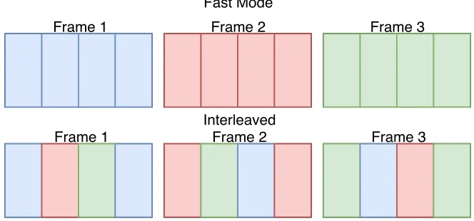
To limit the effect of impulse noise on each frame, a technique called Interleaving can be
employed. Interleaving is the process of taking the potential content of multiple frames of
data, and dividing them into a number of pieces, then sending those pieces mixed together
in frames.
Fast Mode
Interleaved
Frame 1 Frame 2 Frame 3
Frame 1 Frame 2 Frame 3
Figure 2.1: Interleaving
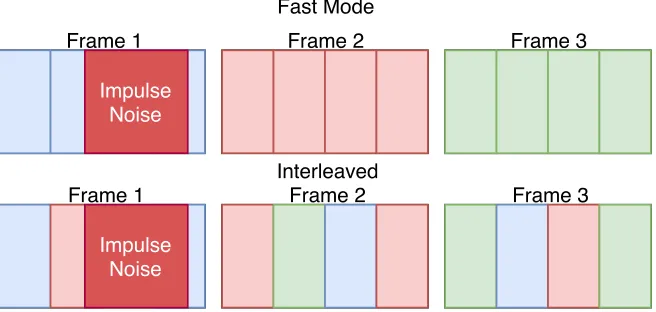
By performing this method of interleaving, the impact of an impulse noise on a single
frame is minimized. Without interleaving, if an impulse noise hit frame one, it would destroy
most of the content of that frame and with that most of the Reed-Solomon code-words that
can be used to repair it. With interleaving, it would destroy a smaller amount of multiple
frames, and less code-words; these small amounts of other frames can be then repaired and
Fast Mode
Interleaved
Frame 1 Frame 2 Frame 3
Frame 1 Frame 2 Frame 3
Impulse Noise
Impulse Noise
Figure 2.2: Interleaving under impulse event
2.5.2.1 Downsides of interleaving
Though interleaving is a very powerful technique for reducing the impact of noise events,
there are significant downsides over fast mode. As data units are received in the DSL
transceiver, there is additional time required to separate these into pieces, and reorder them
interleaved. This process adds significant, direct latency to a DSL connection. This can
make these connections unsuitable for applications such as VOIP, and often lines requiring
VOIP are deployed in fast mode or make use of dual paths (one with fast mode, one with
Interleaving) to operate properly. Interleaving was one of the significant factors enabled in
this study to represent a typical DSL internet deployment.
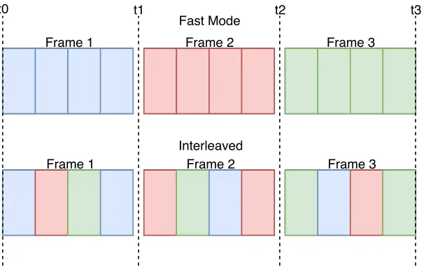
This effect on latency can be seen in Figure 2.3. With fast mode the full content of
Frame one is received at time t1, whereas with interleaving the full content of frame 1 is
not received until time t3. This imposes a significant fixed latency increase. The amount
of interleaving depth is defined by the DSLAM and determines the amount of division of
frames. The example above uses an interleaving depth of 3, where values can range as high
Fast Mode
Interleaved
Frame 1 Frame 2 Frame 3
Frame 1 Frame 2 Frame 3
t0 t1 t2 t3
Figure 2.3: Latency affect from interleaving
2.5.2.2 FEC + Interleaving Settings
DSL defines a huge number of settings to control impulse noise protection settings.
Depend-ing on the level of expected noise on a line, or the use case of said line, these settDepend-ings can be
adapted to meet performance or stability goals.
Impulse Noise Protection Minimum (INP):
The INP parameter is defined in terms of DMT (Discrete Multi-Tone Symbols). DMT
symbols are single unit data frames. The INP parameter is defined as the number of DMT
symbols which can be completely corrected by the FEC systems, regardless of the amount of
errors [4]. The INP setting is not a direct parameter by itself, but rather a guideline for the
FEC system to perform under. Based on INP settings the Reed-Solomon encoding settings
are determined. Values vary between 0 and 16 with 0 indicating that there is no minimum
amount of symbols.
Interleaving Depth:
As defined above, the depth of interleaving is the amount of divisions of each data unit that
is performed by the interleaver. Though this is a configurable parameter by a chipset, from
and not directly configured.
Maximum Interleaving Delay:
The maximum interleaving delay defines the maximum amount of delay placed on the system
by the interleaver between the two DSL interfaces (in one direction). If the interleaver is
disabled (fast mode) the maximum delay between the DSL interfaces may not exceed 2 ms
(in one direction). This value typically ranges between 2 and 63 ms.
2.5.3 Retransmission
Retransmission is a newer method for dealing with packet corruption due to impulse noise
events. This is an optional setting, only supported in newer VDSL2 connections.
When Retransmission is enabled. a DSL transceiver’s unit of data is referred to as
a Data Transmission Unit (DTU) [2]. Retransmission works by attaching a frame check
sequence (FCS), and sequence number, to a DTU and buffering DTU’s before they are sent.
If the FCS fails, or the receiver has missed a transmission (known via sequence number), a
negative acknowledgement is sent indicating that the DTU needs Retransmission and the
receiver awaits a Retransmission from the sender.
2.5.3.1 Impact of Retransmission on Network Performance
Retransmission has benefits in use over traditional FEC methods of noise protection in some
scenarios, though they can be used in conjunction with each other. In some cases it may
allow for lower or no interleaving to be used, while still having protection from impulse
noise. This may lead to a direct increase in available data rate, and improved latency during
low-noise periods.
Retransmission can also have notable downsides, meaning much higher peak latencies
when packets are being frequently retransmitted, while having lower good case average
la-tency when noise events are rare. There is also a large memory requirement to do downstream
physical upgrade to be able to do restransmission.
There is a balance to be struck, if noise events are expected to be very frequent on a line,
Retransmission may be a worse option compared to FEC, if they are relatively infrequent,
better data rate, latency, and there by better user QoS can be achieved without sacrificing
line stability.
2.6 Impact of Noise Protection on Network Performance
All forms of DSL noise protection have some impact on latency, with FEC + Interleaving
being more fixed, consistent impact on latency and Retransmission applying conditional
impact on latency depending on line conditions. In a system where Noise is a factor, there
is no method of noise protection that does not come at some cost.
The maximum cost of latency can depend on the configuration of these parameters; DSL
provides many tools to allow operators to configure these on a case by case basis, but their
use should be carefully considered and weighed based on deployment scenario.
DSL is, in part due to these technologies, a high latency technology that can have heavy
effect on user QoE, especially with the increases in low latency video streaming and gaming
service usage by end users. The various deployment scenarios tested in this study,
experi-enced a wide range of average latency depending on the direction of traffic, and the presence
of noise. This latency existing only in the last mile is additional to all other network latency
CHAPTER 3
DSL Measurements
3.1 Test Setup
To perform our study we decided to use equipment that is representative of the average case
that may deployed in a customer home. All pieces of equipment were carefully chosen to
minimize impact from potential interoperability issues.
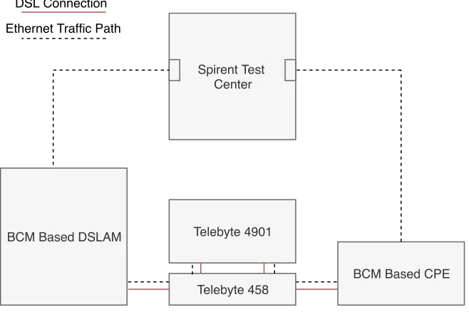
3.1.1 Test Setup
Spirent Test Center
Telebyte 4901
Telebyte 458 BCM Based DSLAM
BCM Based CPE
Ethernet Traffic Path DSL Connection
3.1.1.1 DSLAM
The DSLAM chosen was using a Broadcom based chipset, model 65300, running version
VDSL-5B 16l v10.09.80. This device was configured to bridge untagged traffic from a 1
Gbps copper (Ethernet) SFP in its network port to its DSL interface. Only the line under
test was connected to the DSLAM at any time during testing. This device was chosen
to represent an average DSLAM that would support newer VDSL2 technologies such as
Retransmission.
3.1.1.2 CPE
The CPE was also a Broadcom based chipset model 63138, running version A2pvbH042u.d26q.
This device was chosen to minimize any interoperability issues with no cross-vendor chipset.
This device is available commercially and the version was the newest available at the time.
This device was set to bridge traffic from its DSL interface though its gigabit Ethernet
interface.
3.1.1.3 Traffic generator
The traffic generator chosen was a Spirent Test Center running version 4.75. Both the CPE
and CO sides were connected via a one gigabit copper (Ethernet) SFP.
3.1.1.4 Noise Generator
The noise generator chosen to generate and inject both the fixed level white noise and impulse
noises was a Telebyte 4901. The noise files chosen were generated as part of a library for
Broadband Forum TR-114 and were modeled on real noise encountered in the field.
3.1.1.5 Loop Simulator
The loop simulator was a Telebyte 458-LM-A1-30-TR114 model loop simulator. This was
3.1.1.6 Cabling
All cabling used in this setup was Cat5e or better of less than 6 foot lengths, with the
exception of the connection between the DSLAM and Spirent Test Center was a longer
connection of Cat5e or better quality.
3.1.1.7 Switch
Some test cases involved a switch using port mirroring to capture Wireshark packet captures.
This switch was a Cisco WS-C4948E enterprise grade switch. The switch was tested to add
minimal delay to captures, less than 10 µs. The presence or absence of the switch does not
have a significant effect on the measurements.
3.2 Traffic Details
For this project we chose to test with stateless Ethernet traffic, containing UDP (Unreliable
Datagram Protocol) headers. Ethernet was chosen to remove the impact of stateful traffic
protocols such as TCP potentially affecting the measurement of the DSL connection. For
FEC cases traffic levels were tuned to a percentage of the NDR (net data rate), a value
pro-vided by the DSLAM. For Retransmission cases, traffic levels were tuned to ETR (Expected
Throughput). Cases varied with level using either (0.5 * ETR/NDR) or (0.9 * ETR/NDR)
traffic level, 50% and 90% respectively.
3.2.1 Traffic Used
For this testing we chose to use the standard IMIX (Internet Mix) traffic defined by the
Spirent Test Center. The Test Center allows for configuration of this traffic, though none
was done for this testing. The standard mix provided by the Spirent Test Center is broken
down in Table 3.1.
scenario for a DSL connection, due to the large proportion of small sized frames (meaning
more frames per data rate.) This was chosen to give a more representative case, as real
traffic will include variable sized frames.
IP Total Length (Bytes) Default Ethernet (Bytes) Weight Percentage
48 66 7 57.33%
576 594 4 33.33%
1500 1518 1 8.33%
Table 3.1: Spirent IMix traffic distribution
3.2.2 Spirent Latency Measurement
The Spirent Test Center relies on a time stamping method to measure the latency between
frames. This is included in the payload so it does not add any frame size. This includes a
timestamp, sequence number, and stream ID [7]. The Spirent Test Center was measuring
latency by appending these signatures on the outbound interfaces, and removing them upon
reception, calculating the time in travel at that point. This method means that all
measure-ments should be accurate and have minimal effect from any clock skew. This also means
that all measurements are one way latency, and not round trip times.
3.2.3 Histograms
Following the initial decision to study latency as the focus of these experiments, methods
for measuring latency accurately were looked into. We decided to leverage the Histogram
feature of the Spirent Test Center. This feature allows a user to configure 16 buckets to
group each packet in depending on their measured latency. These buckets were manually
configured to provided good granularity on the measured latency, meaning no one bucket
would have too high of a proportion of the measured traffic. It would be superior to measure
the latency of each frame individually, however, the Spirent Test Center and other tools that
3.3 Setup and Test Procedure
Throughout the measurement campaign, a number of variations of the configuration were
used. These were used to push the DSL line into various states, including many very stressed
cases, providing insight into the functionality of each setting and its impact on latency
performance.
It was initially determined that DSL in a unimpaired condition provided reliable and
steady performance with little latency variation outside of the fixed level provided by the
configuration. These cases were given less focus during the course of the study, with a
more heavy focus placed on studying the more impaired conditions where higher latency
would occur, and the error correction/mitigation technologies would be required for proper
operation.
Many of the test cases chosen were intended to represent the worst cases a consumer DSL
deployment may be able to encounter and survive.
3.3.1 Test Procedure
For all cases the test procedure was static, aside from configuration values:
• The loop simulator was set to the required value for that test case.
• The Noise generator was configured to inject -140 dBm/Hz White Noise, to minimize
the impact of any background lab noise.
• The DSLAM was configured with the line disabled.
• The line was enabled, and the CPE allowed to train and remain stable for 60 seconds.
• The line was measured from the DSLAM and recorded, including performance counters.
• The traffic generator was configured to either 50% or 90% of the NDR reported by the
• Any impairment (REIN Noise) was played on the Noise Generator, remaining enabled
through the test case.
• Test Traffic was enabled in the Spirent Test Center and passed through the setup.
• Test Traffic and Noise were played for 30 seconds.1
• Noise and traffic were ceased.
• Measurements were taken from the DSLAM (line batch, and performance counters)
and results from the Spirent Test Center were saved.
3.3.2 DSL Profiles
For these experiments two differing profiles were used. Both were based on the same
Broad-band forum TR-114 profile. This profile was chosen to represent an average 8 MHz, North
American DSL deployment profile [8]. The settings contained in this profile would be
com-patible across many deployment scenarios and over a range of loops. INP and Interleaving
settings are typical for deployment profiles. The full settings of this profile are defined in
Table 3.6 and Table 3.7
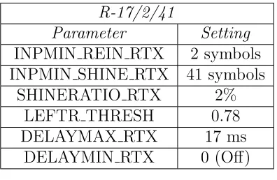
The only variation applied to that profile was the use of a typical Retransmission profile.
The Retransmission profile applied was also of standard settings based on Broadband Forum
TR-249 [9]. Full settings are defined in Table 3.2
1Experiments were performed with longer times to determine testing time. It was determined that 30
R-17/2/41
Parameter Setting
INPMIN REIN RTX 2 symbols
INPMIN SHINE RTX 41 symbols
SHINERATIO RTX 2%
LEFTR THRESH 0.78
DELAYMAX RTX 17 ms
DELAYMIN RTX 0 (Off)
Table 3.2: R-17/2/41 Profile
3.4 Experiment Results
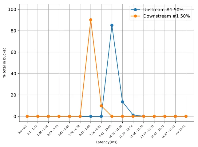
3.4.1 FEC Upstream and Downstream variation
As mentioned in Chapter 2, many of the settings requested by a DSL profile are suggestions
or high level requirements for the behavior of a modem, and often actual settings may differ
from the those requested in the profile.
For example, the default profile used for this experiment requests an identical Maximum
Interleaver Delay of 8 ms, and a minimum INP of 2 symbols. When looking at the
measure-ments recorded from the DSLAM, Actual Interleaver Delay is 5 ms for Downstream, and 8
ms for Upstream, with INP at 2 symbols for both sides. This results in the increased latency
by a fixed amount on the upstream side when compared with the downstream side.
Even under the same configuration settings, actual values can differ from the requested
values as the DSL chipsets attempt to optimize operation under the current conditions. This
is seen with longer loops as the actual interleaver delay increases with no alteration to the
0.0 - 0.1 0.1 - 1.341.34 - 2.592.59 - 3.833.83 - 5.085.08 - 6.326.32 - 7.567.56 - 8.818.81 - 10.0510.05 - 11.2911.29 - 12.5412.54 - 13.7813.78 - 15.0315.03 - 16.2716.27 - 17.51>= 17.51
Latency(ms)
0 20 40 60 80 100
% total in bucket
Upstream #1 50% Downstream #1 50%
Figure 3.2: Upstream and Downstream latency variation, 50% traffic, FEC + Interleaving
3.4.2 50% traffic vs 90% traffic
One initial variation in test setup, was traffic level. Two differing traffic levels were tested,
those being 50% of NDR/ETR (as reported by the DSLAM) and 90% of NDR/ETR. These
variable traffic levels were tested across all configurations and noise impairments.
Cases using 90% traffic levels had more distributed latency, with higher peak and average
latency measurements. This variation is likely due to the high volume of packets causing
filled buffers within the transceivers. Both 50% and 90% measurements were continued
through most of the campaign. It was suspected that 50% traffic levels may better indicate
the real use case of a users connection, and 90% traffic was more accurate to model the worst
case a connection might encounter. Performance in the Retransmission enabled cases looked
0.0 - 0.1 0.1 - 1.341.34 - 2.592.59 - 3.833.83 - 5.085.08 - 6.326.32 - 7.567.56 - 8.818.81 - 10.0510.05 - 11.2911.29 - 12.5412.54 - 13.7813.78 - 15.0315.03 - 16.2716.27 - 17.51>= 17.51
Latency(ms)
0 20 40 60 80 100
% total in bucket
Upstream #1 50% Downstream #1 50% Upstream #3 90% Downstream #3 90%
Figure 3.3: 50% Traffic vs 90% Traffic, FEC + Interleaving
Value US 50% US 90% DS 50% DS 90%
TX Count 88,664 150,585 269,652 486,082
RX Count 88,664 150,585 269,652 456,082
Dropped Count 0 0 0 0
Avg Latency (ms) 9.69 11.30 7.29 7.82
Min Latency (ms) 9.12 9.15 6.86 6.94
Max Latency (ms) 13.94 25.18 8.91 14.48
Table 3.3: Comparison of 50% to 90% traffic level, FEC + Interleaving
3.4.3 Impulse Noise
For impulse noise, three levels of interference were tested. These three levels being white
noise only (control), 100 µs REIN, and 1 ms REIN. As is expected, all of these levels of
interference resulted in packet destruction and longer latency (in Retransmission cases). It
was determined that only the Retransmission settings used had the correct amount of
pro-tection required to survive REIN noises as long as 1 ms. It is possible with more interleaving
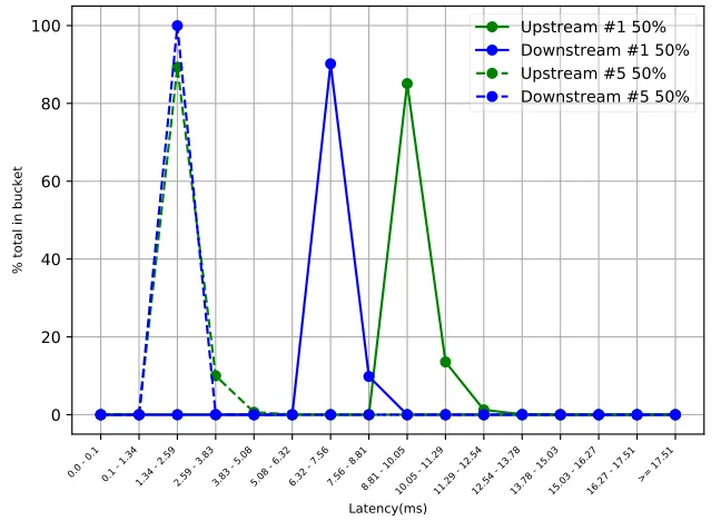
3.4.3.1 Retransmission vs FEC + Interleaving
Perhaps the most major difference in configuration attempted in this study, was the inclusion
and removal of Retransmission. When Retransmission is applied, the line was found to enable
no additional protections (meaning it was running in fast mode). This resulted in lower
latency, and often higher data rates, under good conditions (as no interleaving was present.)
This would provide a notable performance increase to a customer using this connection.
0.0 - 0.1 0.1 - 1.341.34 - 2.592.59 - 3.833.83 - 5.085.08 - 6.326.32 - 7.567.56 - 8.818.81 - 10.0510.05 - 11.2911.29 - 12.5412.54 - 13.7813.78 - 15.0315.03 - 16.2716.27 - 17.51>= 17.51
Latency(ms)
0 20 40 60 80 100
% total in bucket
Upstream #1 50% Downstream #1 50% Upstream #5 50% Downstream #5 50%
Figure 3.4: FEC (#1) vs Retransmission(#5), 50% traffic
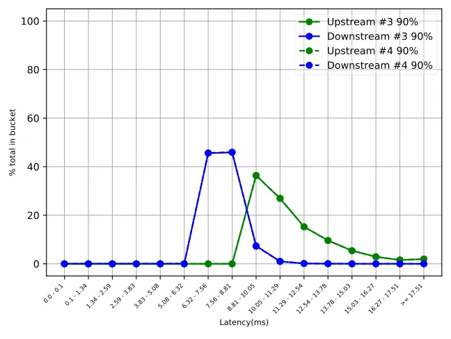
During impulse noise cases, clear differences between Retransmission and FEC approaches
became apparent. With FEC + Interleaving, under the 100 µs length REIN events, some
packets may be lost, but the overall latency performance was not significantly affected. Any
REIN noise longer than 100 µs would cause a drop in line sync, as the protection was
inadequate to repair the frames damaged by the REIN event. This is typical of FEC +
Interleaving, as the additional latency and overhead required to repair the damaged frames,
was present at configuration time; meaning that no additional latency is incurred during
REIN events.
0.0 - 0.1 0.1 - 1.341.34 - 2.592.59 - 3.833.83 - 5.085.08 - 6.326.32 - 7.567.56 - 8.818.81 - 10.0510.05 - 11.2911.29 - 12.5412.54 - 13.7813.78 - 15.0315.03 - 16.2716.27 - 17.51>= 17.51
Latency(ms)
0 20 40 60 80 100
% total in bucket
Upstream #3 90% Downstream #3 90% Upstream #4 90% Downstream #4 90%
Figure 3.5: FEC Control (#3) vs 100us REIN (#4) (Lines are overlapping)
As the Retransmission equipped line saw REIN noise events, increased latency was seen as
packets were re-transmitted. Both 100µs and 1 ms REIN events were found to be survivable
for the Retransmission equipped line, though significant packet drop was observed under 1
ms events, in addition to very high latency.
Both of these technologies demonstrate a different approach to noise protection. With
FEC + Interleaving the line is correcting forward of the event occurring, and the latency
and bandwidth cost is paid up-front and is a consistent and fixed cost. With Retransmission
the cost of protection is paid as the events occur and improved latency can be seen during
the quiet periods. This study also observed significantly higher peak latency under the
Retransmission case, even under equivalent noise events (25 ms vs 35 ms for the 100 µs
case).
It is also notable that in several cases, Retransmission resulted in a higher data rate, as
line in good scenarios, which would provide improved performance for many low latency
services a customer may use, without sacrificing the ability to remain online during noise
events.
0.0 - 0.1 0.1 - 1.341.34 - 2.592.59 - 3.833.83 - 5.085.08 - 6.326.32 - 7.567.56 - 8.818.81 - 10.0510.05 - 11.2911.29 - 12.5412.54 - 13.7813.78 - 15.0315.03 - 16.2716.27 - 17.51>= 17.51
Latency(ms)
0 20 40 60 80 100
% total in bucket
Upstream #8 90% Downstream #8 90% Upstream #9 90% Downstream #9 90% Upstream #10 90% Downstream #10 90%
Figure 3.6: Retransmission, 90% traffic, Control(#8), 100µs REIN (#9), 1 ms REIN (#10)
3.4.4 Long Loop Cases
The final variation of the experiment was based around lower data-rates. The intention was
to replicate scenarios present in subscriber networks where a home may be located further
away from a DSLAM, resulting in lower achievable rates. Two loop configuration settings
were determined for use in this scenario, one with approximately 15 Mbps downstream
speeds, and approximately 8 Mbps downstream speeds. To achieve these rates, loops of
approximately 5,750 ft were used for the 15 Mbps case, and loops between 7,300 to 7,500 ft
were used tor the 8 Mbps case. The intention of these settings was to provide an indication
of what a customer could expect over a connection under reasonable access speeds.
In all scenarios with longer loop lengths, more variable latency was observed. Each link,
upstream latency. Following the conclusion of this study, we determined that the very long
latency packets (resulting in much of the data outside the measurement range, may have
been anomalous, and perhaps the result of a configuration issue in those test cases. This was
observed consistently during the course of this study, and more research may be required
to fully characterize the behavior of DSL under long loop scenarios, and to look into the
presence of these very long latency packets. Data outside of these very high values appears
to be accurate to actual performance.
3.4.4.1 FEC + Interleaving
For the DSL connection running FEC + Interleaving, the line was observed to train with a
higher level of interleaving delay (8 ms downstream, 7 ms upstream) when compared to the
short loop cases. This resulted in a fixed amount higher latency than the short loop case.
Long loop cases were initially observed to experience significantly latency values compared
to their short loop counter parts, as well a larger variance.
0.0 - 0.1 0.1 - 1.341.34 - 2.592.59 - 3.833.83 - 5.085.08 - 6.326.32 - 7.567.56 - 8.818.81 - 10.0510.05 - 11.2911.29 - 12.5412.54 - 13.7813.78 - 15.0315.03 - 16.2716.27 - 17.51>= 17.51
Latency(ms)
0 20 40 60 80 100
% total in bucket
Upstream #1 50% Downstream #1 50% Upstream #40 50% Downstream #40 50%
Short Loop US Long Loop US Short Loop DS Long Loop DS
Avg. Latency (ms) 11.30 14.60 7.82 10.30
Min Latency (ms) 9.15 10.30 6.95 9.65
Max Latency (ms) 25.18 62.60 14.50 15.14
Table 3.4: Comparison of 90% traffic, FEC + Interleaving short loop vs Long Loop perfor-mance indicators
3.4.4.2 Retransmission
For the Retransmission enabled case, similar performance to the FEC case was observed.
Higher latency overall, as well as a bi-modality in the upstream direction, and more variable
latency. Latency performance again was much more variable between frames (higher
jit-ter). As suggested above, the presence of these very long values, may have been anomalous
behavior and not indicative of the behavior of all devices under these conditions.
0.0 - 0.1 0.1 - 1.341.34 - 2.592.59 - 3.833.83 - 5.085.08 - 6.326.32 - 7.567.56 - 8.818.81 - 10.0510.05 - 11.2911.29 - 12.5412.54 - 13.7813.78 - 15.0315.03 - 16.2716.27 - 17.51>= 17.51
Latency(ms)
0 20 40 60 80 100
% total in bucket
Upstream #8 90% Downstream #8 90% Upstream #37 90% Downstream #37 90%
Short Loop US Long Loop US Short Loop DS Long Loop DS
Avg. Latency (ms) 3.54 16.60 2.11 2.79
Min Latency (ms) 1.60 2.72 1.41 1.42
Max Latency (ms) 16.05 110.73 6.076 11.66
Table 3.5: Comparison of 90% traffic, Retransmission short loop vs Long Loop performance indicators
3.4.4.3 Measurement Resolution
During the initial study of these cases, it was determined that the window sizing of the
histogram was not adequate to measure the range of values present in these cases. Many
of these cases were repeated with wider histogram windows, and varying histogram window
between the upstream and downstream directions. Those repeated cases were ultimately
used in the modeling of these connections.
The performance of all long loop cases was found to have higher latency than their low
loop counterparts. To fully explain the behavior of these cases, a full mapping and study of
the network performance of these lines under a variety of line conditions and loop lengths
would need to be performed. The focus of the study would need to fully map the performance
of lines under long loop conditions and determine if these long loop cases experience these
very long latency packets.
3.4.4.4 Possible Issues with Long Loop Data
During a cursory re-examination of the data captured in this study, we determined that
the very long latency experienced by both the FEC + Interleaving lines as well as the
Retransmission lines in the long loop case study may have been anomalous. The behavior
of the line with the exclusion of those long latency packets, (those located mostly in the
final bucket), appears consistent with additional test cases run after the conclusion of this
study. A full mapping of long loop cases providing an examination into this issues must be
A cursory look into long loop performance done after the initial study, suggests that the
presence of a bi-modal upstream (likely due to variations in packet size), and overall lower
latency with less extreme maximums is normal for long loops cases. A comparison of a 0 ft
loop vs a 7,000 ft loop from additional data gathering efforts can be seen in Figure 3.9
This test case poses a similar performance to the initial Retransmission test cases, but
does not experience the presence of long latency values outside of the measurement range.
>= 1.0 1.0 - 2.0 2.0 - 3.0 3.0 - 4.0 4.0 - 5.0 5.0 - 6.0 6.0 - 7.0 7.0 - 8.0 8.0 - 9.0 9.0 - 10.010.0 - 11.011.0 - 12.012.0 - 13.013.0 - 14.014.0 - 15.0 >= 15.0
Latency(ms)
0 20 40 60 80 100
% total in bucket
Upstream #1 50% Downstream #1 50% Upstream #8 50% Downstream #8 50%
Figure 3.9: Retransmission, 50% traffic, 0 ft loop, 7,000 ft loop
3.5 Summary
One of the most major parts of this study was this DSL mapping procedure. Performing
these experiments lead to the affirmation of many expectations (such a fixed latency on FEC
configurations and more variable latency on Retransmission configurations.)
The very high levels of latency experienced by a variety of the connections, particularly
the restransmission under REIN events, is indicative of possible serious issues that can be
encountered in deployments worldwide. Many of these levels would be seriously impactful
One avenue for further study is a more complete mapping of how these variations on
parameters (loop length, varying levels of interleaving,) affect latency. This study attempts
only a cursory and partially representative investigation of some worst case scenarios, but
does not attempt to represent the full range of possibilities a DSL connection can encounter.
In addition to that, a deep look into the performance of loop cases would be valuable to
study the presence or absence of the very long latency values seen in the initial study.
Raw data and additional information for the experiments performed in this study are
TR-114 AA8d I 096 056
DSL Parameter Requested Value
xDSL Transmission System(s) Enabled G993 2 A
VDSL2 Limit Mask (includes US0 mask) Annex A, D-32
VDSL2 Profile 8d
Upstream PSD Mask (G.992.3/5 Annex J/M) 0
Max SNRM Upstream (dB) 31
Upshift SNRM Upstream (dB) 30
Target SNRM Upstream (dB) 6
Downshift SNRM Upstream (dB) 1
Min SNRM Upstream (dB) 0
Upshift Time Upstream (seconds) 60
Downshift Time Upstream (seconds) 60
Max SNRM Downstream (dB) 31
Upshift SNRM Downstream (dB) 30
Target SNRM Downstream (dB) 6
Downshift SNRM Downstream (dB) 1
Min SNRM Downstream (dB) 0
Upshift Time Downstream (seconds) 60
Downshift Time Downstream (seconds) 60
Maximum Nominal Transmit Power Upstream (dBm) 14.5
Maximum Nominal Transmit Power Downstream (dBm) 14.5
TR-114 AA8d I 096 056
DSL Parameter Requested Value
Rate Mode (Manual, At-Init, Dynamic) At-Init
Min Rate Upstream (kbps) 128
Max Rate Upstream (kbps) 56,000
Min INP Upstream (symbols) 2
Max Interleaving Delay Upstream (ms) 8
Min Rate Downstream (kbps) 256
Max Rate Downstream (kbps) 96,000
Min INP Downstream (symbols) 2
Max Interleaving Delay Downstream (ms) 8
ForceINP (true/faluse) TRUE
Minimum Reserved Overhead bit-rate (kbps) 16
Trellis Coding Enabled (true/false) TRUE
Bit-swapping Enabled (true/false) TRUE
UPBO Disabled (true/false) FALSE
Force Electrical Length (true/false) FALSE
UPBO A-value US0 40
UPBO B-value US0 0
UPBO A-value US1 53
UPBO B-value US1 21.2
UPBO A-value US2 54
UPBO B-value US2 18.7
UPBO A-value US3 54
UPBO B-value US3 18.7
DPBO Disabled (true/false) TRUE
CHAPTER 4
NetEm Models
4.1 What is NetEm
According to the NetEm web page, NetEm is an enhancement of the Linux traffic control
facilities that allow to add delay, packet loss duplication and more other characteristics to
packets outgoing from a selected network interface [11]. Essentially it is a tool to allow for
basic simulation of network connections by traffic shaping through Ethernet ports on a Linux
machine.
4.2 NetEm Capabilities
NetEm supports a number of parameters in both simple and more complex formats. It has
support for fixed and dynamic delay, packet loss, packet duplication, and packet corruption.
The most complex parameter is delay, supporting three modes, fixed, random variation, and
variation according to an input distribution. Delay can be used to model latency. The
simplest commands allow a fixed delay percentage to be set.
tc qdisc add dev eth0 root netem delay 100ms
This adds a fixed delay to each packet of 100 ms. Either random variation, or random
variation with a simulated correlation to the delay distribution can also be specified. While
this adds some realism, the distribution mode of operation was most important for the
Outside of specifying the delay values and variations, a distribution argument can also be
included. There are a few predefined distributions (uniform, normal, pareto, and
paretonor-mal.) This can be useful and rely on the other delay arguments to center themselves. For
example when using the following command:
tc qdisc change dev eth0 root netem delay 100 ms 20 ms distribution normal
This follows a normal distribution with a mean at 100 ms and a random variation (jitter)
per packet of 20 ms. When the distribution argument is not specified, it defaults to normal,
and all packets would range between 80 ms and 120 ms.
NetEm also allows for custom distribution files to be specified. The maketable program
defined in iproute2, allows a user to generate these distribution files. The input file to this
program is simply a flat list of measurement values. For example:
If a few packets are measured at 10 ms, 12 ms, 13 ms, 14 ms, the input file would be a
file containing 10, 12, 13, 14. (Separated by new lines, not commas.)
This would be passed as input to the iproutemaketable program which would generate
a distribution based around the occurrence of these numbers. This can handle a large
volume of measurements and produce a fairly accurate distribution based around the exact
measurements provided. The table is generally a set of negative or positive numbers, allowing
the distribution to still follow the passed in mean and standard deviation.
In addition to delay based features NetEm supports a full range of other networking
properties. Packet loss can be specified as a simple percentage argument, or a percentage
with an additional correlation value to simulate multiple packet losses due to some event.
NetEm can also specify packet corruption, reordering, and duplication events on a simple
4.3 What to model in DSL
When modeling a network connection, a few parameters are considered, packet loss,
dupli-cation, reordering, as well as latency and bandwidth.
When packet loss is considered, DSL is a generally reliable connection, any packet sent
will be either recovered or resent if it is lost (depending on FEC + Interleaving versus
Retransmission support). Serious packet loss only occurs in the most stressed situations
(such as heavy REIN), and when a link is overrated (more traffic being sent than a line can
support.) Though packet delivery is reliable, latency may be variable under these conditions
depending on the type of noise protection being used. Duplication and reordering events are
also not seen in a typical DSL connection.
Packet corruption is a normal part of DSL. It happens frequently but the aim of
Retrans-mission and FEC is to correct these packet corruptions and replace or resend any corrupted
data. The frequency of these corruptions is dependent on line conditions (presence of noise,
cabling issues). These corruptions are present in our measurements of the DSL line, but
would not be seen from a network perspective (they are corrected by the DSL), so no
addi-tional simulation is necessary by NetEm.
Throughput is one key parameter in modeling a DSL connection. In a DSL connection the
throughput, in the form of upstream/downstream net data rate, is either a directly configured
parameter by a service provider, or a deterministic quality based on line condition, distance
from the termination point, and electrical bandwidth profile. This is generally a tightly
controllable parameter for a DSL connection, and less focus can be given to modeling this
as it should be fairly consistent based on loop length, noise condition, and SNR parameters.
Likely the most key part of the network performance of a DSL connection, and the one
directly modeled by this study, is the latency of the connection. DSL due to the interleaving
or Retransmission of data, and the potential latency of long loops, has increased latency over
Retransmission was chosen as the direct target for modeling, due to its potential impact on
end user QoE and highly variable performance in the DSL measurements.
4.4 Modeling DSL with NetEm
From the measurements gathered during the DSL measurement campaign, it was determined
early on that modeling DSL connections as a whole with a single model was not feasible due
to the highly variable nature of the latency distributions measured. Instead, the target was
to create a number of models and NetEm profiles based around different measured DSL
connection conditions. This would allow the end user of the models to test under a variety
of conditions with the best possible accuracy.
It was also determined that data rate could be simply modeled by using a fixed limit.
Each model was measured at a certain data rate during the DSL testing, but the model
could be simply set to that limit with a simple NetEm command, no more sophisticated
modeling was required. DSL in most connections provides a fairly steady data rate with
little fluctuation, depending on the features enabled on a line.
The modeling of the latency of a connection was a more involved task. The distribution
of the latency varied highly depending on the conditions of the line and the overall length
of the cabling, or presence of noise. Generally, in a well behaved connection free of any
impairment, (added noise corrupting packets and causing either Retransmissions or FEC
events), latency was relatively consistent. In these cases latency followed a very tight normal
distribution around a fixed value. This can be seen in the DSL measurements.
A higher focus was given to highly impaired cases, such as those experiencing significant
REIN noises. During the measurement campaign it was found that these cases would often
result in very high and highly variable latency, and would be very disruptive to any service
running over these connections. The connections were targeted for the majority of the
modeling effort.
distribution models were fruitless, and it was quickly determined that custom distribution
files would be required.
Given the limitation of measurement tools used, only histograms of latency values could
be gathered in the DSL campaign. These histogram buckets (16 total, on each side of a
connection), were tuned as close as possible to provide the best resolution for each particular
test case’s latency distribution. Since the input of the NetEm table generator is raw numbers,
some effort was required to convert the bucket sizes and counts to actual number values.
To accomplish the task of converting buckets to raw values, a simple script was
imple-mented in Python to create raw data files. This script worked naively and placed the average
value of the upper and lower bound of each particular bucket serially into a file. This raw
file was able to be input into the iproute2 table creator which resulted in a distribution
file. Both an upstream and downstream distribution file was created for each set of NetEm
models. The mean and standard deviation of the values in the buckets were also calculated
and those values used as additional parameters into the NetEm model.
These models were then turned into a set of commands for an interface. These commands,
with their corespondent files, would allow a typical linux server bridging traffic from one
interface to another, to apply the commands via NetEm to their interfaces and shape the
traffic, resulting in similar impact on the traffic to the DSL link it was simulating. Each
model had four commands.
1. tc qdisc change dev enp3s0f0 root handle 1:0 netem delay 7062us 370us 0\%
distribution no_rtx_control_1DOWN
2. tc qdisc change dev enp3s0f1 root handle 1:0 netem delay 9631us 509us 0\%
distribution no_rtx_control_1UP
3. tc qdisc change dev enp3s0f0 parent 1:1 pfifo limit 1000
4. tc qdisc change dev enp3s0f1 parent 1:1 pfifo limit 1000
Command 1, is the shaping command for the downstream side of the connection, interface
for this configuration to be applied to. The next part of the command ”delay 7062us 370us
8%” referes to the delay parameters, being mean (7062µs), standard deviation (370 µs), and
co-dependancy factor (correlation between each frame and its previous frames.) which for our
purposes was 0%. The final part of the command ”distribution no rtx control 1DOWN”
is specifying to use a custom distribution file, name ”no rtx control 1DOWN”. Command 2
is identical to command one, but for the upstream interface.
Commands 3 and 4 are to specify that NetEm use pfifo queuing, with a 1000 packet limit
to shape the traffic. This was to attempt to not only ensure a consistent queuing method
was used, but to attempt to minimize packet reordering. Ultimately, this command was
ineffectual in producing non-reordered traffic, but was left in to ensure that a consistent
method was used.
Models of this style were created for every relevant link, and were tested and compared
CHAPTER 5
Model Results and Comparison
5.1 Test Setup
Spirent Test Center Test Traffic Path
Linux Server Running NetEm Model
Figure 5.1: NetEm Measurement Test Setup
The NetEm experimental setup involved the same traffic generation hardware as the DSL
setup, and the same level of traffic was run through each simulated link case. The hope of
the experiment was that the network traffic would perform identically to the DSL it was
simulating, returning a latency distribution across the histogram.
5.1.0.1 Hardware Setup
All NetEm tests were run on an Ubuntu based server, running Ubuntu 16.04.2 LTS. This
server had an Intel Pentium(R) Dual-Core CPU E5300 running at 2.6 Ghz, 4 GB of DDR2