Parameter estimation of the modified Weibull model
based on grouped and censored data
Mazen Zaindin
Department of Statistics and O.R., Faculty of Science, King Saud University, P.O. Box 2455,Riyadh 11451, Saudi Arabia.
E-mail: [email protected]
Abstract
--
This paper presents estimations of the modified Weibull distribution model based on grouped and censored data. The maximum likelihood method is utilized to derive point and asymptotic estimates of the unknown parameters. confidence and Further, the asymptotic confidence intervals for the parameters are derived from the Fisher information matrix. The likelihood ratio test is applied to test the goodness of fit of the modified Weibull distribution. To illustrate the application of this new distribution, a set of real data is analyzed.Index Term
--
modified weibull distribution, grouped data, maximum likelihood method.1. INTRODUCTION
Estimation of the unknown parameters of statistical distributions is one of the most important problems facing applied statisticians. This paper presents estimations of the unknown parameters of the modified Weibull distribution model based on grouped and censored data. The modified Weibull distribution has been introduced by Sarhan and Zaindin (2009)[6]. This distribution generalizes the exponential, Rayleigh, linear failure rate and Weibull distributions. These distributions are the most commonly used distributions in reliability and life testing since, they have several desirable properties and nice physical interpretations [2]-[5]. Unfortunately the exponential distribution has only constant failure rate and the Rayleigh distribution has increasing failure rate. The linear failure rate distribution generalizes both these distributions which may have non-increasing hazard function,[7]. Also, the Weibull distribution generalizes exponential and Rayleigh distributions. It may have an increasing or decreasing failure rate. For the case when it has an increasing failure rate, its failure rate function starts from the origin. This property limits its application in practice. The modified Weibull distribution that generalizes all the above distributions can be used to describe several reliability models. It has three parameters, two scale and one shape parameters. Notation of MWD(α,β,γ) is used to denote the modified Weibull distribution with three parameters α ,β and γ.
In reliability analysis, tests can be performed for units or systems either on complete data or grouped data. Tests on grouped data are more frequently, since they, generally, cost less and require fewer efforts. Moreover, they are sometimes the only possible or available for units or their systems [1].
The aim of this paper is to estimate the unknown parameters of the modified Weibull distribution based on grouped and censored data. The maximum likelihood method is used to derive point and asymptotic confidence estimates of the unknown parameters.
The model was provided on real data to test whether it fits these real data better than other models. The rest of the paper is organized as follows. In Section 2, definition and some characteristics of the modified Weibull distribution are presented. Point estimation and interval estimations of the unknown parameters are discussed in Section 3. In Section 4 an illustrative example is presented to explain how the modified Weibull distribution fits a set of real data better than other distributions. A conclusion is drawn in Section 5.
2. THE MWD
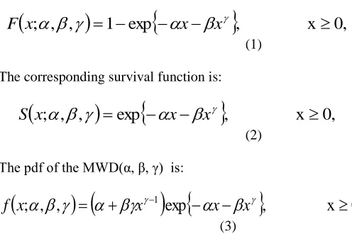
The cdf of MWD(α, β, γ) takes the following form:
x
;
,
,
1
exp
x
x
,
x
0,
F
(1)
The corresponding survival function is:
x
;
,
,
exp
x
x
,
x
0,
S
(2)
The pdf of the MWD(α, β, γ) is:
x
;
,
,
x
1
exp
x
x
,
x
0,
f
(3)
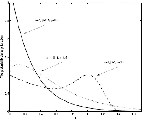
Fig. 1. Different patterns of the probability density function
The hazard rate function of MWD(α, β, γ) is
;
,
,
1
,
x
0,
x
x
h
(4)
Fig. 2 shows different patterns of the hazard rate function.
Fig. 2. Different patterns of the hazard rate function
This distribution generalizes the following distributions: 1. Exponential distribution, ED(α) when β=0; 2. Raleigh distribution, RD(β) when α=0, γ = 2; 3. Linear failure rate distribution, LFRD(α, β) when γ =
2; and
4. Weibull distribution WD(β, γ) when α = 0.
The mean time to failure of the modified Weibull distribution:
0
1
1
1
!
1
1
i
i
i
i
i
MTTF
3. PARAMETERSESTIMATION
Consider n independent and identical components put on test. Assume that the lifetimes of these components follow the modified Weibull distribution expressed in the previous
section. Let t=t1,t2,…tk, ,where t1<t2<… <tk, denote the predetermined inspection times
with tk representing the completion time of the test. Also, let
t0=0 and tk+1= ∞. For i=1,...,k, denote by ni the number of failures recorded in the time interval (ti-1, ti) and by nk+1 the number of censored units, that is units that have not failed by the end of the test.
3.1 Maximum Likelihood Estimators
Using the data described above, the likelihood function is given by:
ki
n k ni
i i
k
t
T
P
t
T
t
P
C
t
L
1 1
1
,
(5) Where
1
1
! !
k
i i
n n C
is a constant with respect to the parameters α, β and γ. Since,
t
i1
T
t
i
F
t
i
F
t
i1P
and
T
t
k
F
t
kP
1
therefore, (5) can be written as
k
i
n i i
n k
i k
S
t
S
t
t
S
C
t
L
1 1
1
,
(6) where θ= (α, β , γ).
substituting (2) into (6), one gets
ki
n i i i
i n
k k
i k
t
t
t
t
t
t
C
t
L
1
1
1
exp
exp
exp
,
1
i i i i i n k kk
t
t
n
t
t
t
t
n
C
t
kexp
exp
ln
ln
,
1 1 1 1
We let
1
1
,...,
1
0
0
k
i
if
k
i
if
e
i
if
A
ti tii
writing simply, Ai(θ) by Ai, the partial derivatives of ℓ are
ki i i
i i i i i k k
A
A
t
A
t
A
n
t
n
1 1 1 1 1
(7)
ki i i
i i i i i k
A
A
t
A
t
A
n
t
n
k 1 1 1 1 1
(8)
ki i i
i i i i i i i k k
A
A
t
t
A
t
t
A
n
t
t
n
k 1 1 1 1 1 1 1ln
ln
ln
(9) Setting,
0
and
,
0
,
0
we get the likelihood equations, which should be solved to get the MLE of the parameters α, β and γ. As it seems the likelihood equations have no closed form solutions in α, β and γ. Therefore, numerical technique method was used to get the solution.
3.2 Asymptotic confidence bounds
Since the MLE of the element of the vector of the unknown parameters θ=(α,β,γ), are not obtained in closed forms, then it is not possible to derive the exact distributions of the MLE of these parameters. Thus, we derive approximate confidence intervals of the parameters based on the asymptotic distributions of the MLE of the parameters. It is known that
the asymptotic distribution of the MLE
is given by see Miller(1981)[9],
12
0
,
N
I
Where
I
1
is the variance covariance matrix of the unknown parameters θ=(α,β,γ). The elements of 3×3 matrix1
I
,I
ij
i,j=1,2,3, can be approximated by
ijI
, where
j i ijI
2From (7) through (9), the second partial derivatives of the log-likelihood function are found to be
ki i i
i i i i i
A
A
t
t
A
A
n
1 2 1 2 1 1 2 2
ki i i
i i i i i i i i i
A
A
t
t
t
t
t
t
A
A
n
1 2 1 1 1 1 1 1 12
ki i i
i i i i i i i i i i i i i
A
A
t
t
t
t
t
t
t
t
t
t
A
A
n
1 2 1 1 1 1 1 1 1 1 1 2ln
ln
ln
ln
ki i i
i i i
A
A
t
t
A
A
n
i i1 2 1 2 1 2 2 1
21 1 1 2 1 2 1 1 1 1 1 1 1 1 1 2
/
}
ln
ln
1
ln
1
ln
ln
ln
{
i i i i i i i i i i i i i i i i i i k i i i i i i i iA
A
t
t
A
t
t
A
t
t
t
A
A
t
t
t
A
A
t
t
t
t
A
A
n
21 1 2 1 2 1 2 1 1 1 2 1 1 1 1 2 1 1 2 2
/
}
ln
ln
ln
ln
2
1
ln
1
ln
{
i i i i i i i i i i i i i i i i i i i k i i i i i i iA
A
t
t
A
t
t
A
t
t
t
t
A
A
t
t
t
A
A
t
t
t
A
A
n
,
,
,
1112 1
11 2 1
11 2
Z
I
Z
I
Z
I
(10)
Here, Zα/2 is the upper (α/2)th percentile of the standard normal distribution.
4. DATA ANALYSIS
In this section we use a set of real data presented by Nelson in [8], which reports a set of cracking data on 167 independent and identically parts in a machine. The test duration was 63.48 months and 8 unequally spaced inspections were conducted to obtain the
number of cracking parts in each interval. The data were
(t1,…t8) = (6.12, 19.92, 29.64, 35.4, 39.72, 45.24, 52.32, 63.48) and
(n1,…,n9)=(5, 16, 12, 18, 18, 2, 6, 17, 73).
We assume that these data follow different distributions. Besides the modified Weibull distribution MWD (α,β,γ), the distributions considered here are:
Exponential with parameter, α , ED(α). Its survival function is:
t
e
t,
t
0,
0
S
Weibull distribution with parameters β and γ , WD(β,γ). Its survival function is
t
e
t,
t
0,
0,
0
S
Raleigh distribution with parameter β, RD(β). Its survival function is
,
t
0,
0
22
t
e
t
S
Linear failure rate distribution with parameters α and β ,
LFRD(α, β). Its survival function is
,
t
0,
0,
0
22
tt
e
t
S
First, we compute the maximum likelihood estimator(s) for the parameters included in each distribution. Then we compare these distributions according to two different criteria. The criteria used are: the log-likelihood function and the least square deviation Q of the survival functions of the above mentioned distributions from the empirical survival function. Finally, we compute the asymptotic confidence intervals of the parameters of the underlying distribution and the
maximum likelihood estimate of the MTTF of each distribution.
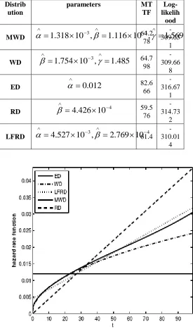
Table I shows the MLE of the parameter(s) and MTTF of the distributions considered and the associated log-likelihood function value.
TABLE I
THE MLE OF THE PARAMETER(S), MTTF AND THE LOG-LIKELIHOOD FUNCTION
Distrib ution
parameters MT
TF
Log-likelih
ood
MWD
1
.
318
10
3,
1
.
116
10
3,
1
.
569
64.278 -309.65
1
WD
1
.
754
10
3,
1
.
485
64.798 -309.66
8
ED
0
.
012
82.666 -316.67
1
RD
4
.
426
10
4
59.576 -314.73
2
LFRD
4
.
527
10
3,
2
.
769
10
4
61.4-310.01
4
Fig. 3. The hazard rate functions
Fig. 3 shows the fitted hazard rate functions of the WD(1.754×10-3,1.485), ED(0.012), RD(4.426×10⁻⁴), LFRD(4.527×10⁻³, 2.769×10⁻⁴) and MWD(1.318×10⁻³, 1.116×10-3,1.569).
The variance covariance matrix of MWD(1.318×10⁻³, 1.116×10-3,1.569) is computed as
173
.
0
10
871
.
9
10
06
.
2
10
871
.
9
10
707
.
5
10
231
.
1
10
06
.
2
10
231
.
1
10
007
.
3
4 3
4 6
5
3 5
5 1
I
Thus, the variances of the MLE of α, β and γ become
5
10
007
.
3
Var
,5
.
707
10
6
Var
and173
.
0
Var
. Therefore, the 95% C.I. of α, β and γ,respectively, are [0, 0.012], [0, 5.799×10⁻³] and [0.754, 2.384].
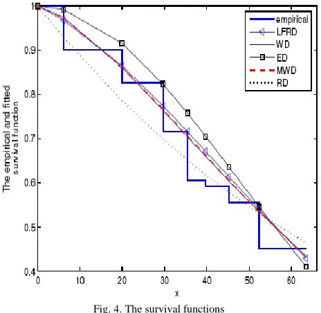
The survival function of the data is estimated using parametric and parametric methods. In the case of the non-parametric estimation, we used Kaplan-Meier method. For the parametric estimations, we used the above mentioned distributions. Fig. 4 shows the results of these estimations.
Fig. 4. The survival functions
Also, we computed the least square deviations. The values of these statistics are summarized in table II below.
TABLE II
THE LEAST SQUARE DEVIATIONS Q
Distribution MWD WD ED RD LFRD
Q 0.1009 0.1011 0.667 0.513 0.104
5. CONCLUSIONS
The parameter estimation of the modified Weibull distribution with three unknown parameters α, β and γMWD(α β,γ), based on grouped and censored data is discussed in this paper. The maximum likelihood technique has been used to derive both point and interval estimations of the three unknown parameters α, β and γ. We tested the MWD(α β,γ) against
ED(α), WD(β,γ), RD(β) and LFRD(α β) using a set of real data from Nelson(1982). Based on the two criteria (the values of the log-likelihood function and least square deviations), we found that the MWD(1.143 ×10⁻³, 1.143×10⁻³, 1.565) has the least values among all distributions and, therefore fits the data better than other mentioned distributions.
REFERENCES
[1] Ehrenfeld, S. (1962). Some experimental design problems in attribute life testing, J. Amer. Statistical Assoc., 57, 668-679
[2] Barlow, R. E. and Proschan, F. (1981). Statistical Theory of Reliability and Life Testing, To Begin With, Silver Spring, MD.
[3] Burr, I.W. (1942). Cummulative frequency function, Ann. Math. Statist. Vol. 13, 215-232.
[4] Genedenko, B.V., Belyayev, Y.K. and Solovyev, A.D. (1969). Mathematical Methods of Reliability Theory, Academic Press, New York.
[5] J. F. Lawless, "Statistical Models and Methods for Lifetime Data," John Wiley and Sons, New York, 2003.
[6] Sarhan, A.M., and Zain-din, M., Modified Weibull distribution, Applied Sciences, vol.11, pp. 123-136, 2009
[7] L. J. Bain, Analysis for the Linear Failure-Rate Life-Testing Distribution, it Technometrics, Vol. 16, no. 4, pp. 551-559, 1974. [8] W. Nelson, Applied life data analysis, John wiley, NewYork,
1982.