Monte Carlo methods
Rémi Bardenet
1Department of Statistics, Oxford University
Abstract. Bayesian inference often requires integrating some function with respect to a
posterior distribution. Monte Carlo methods are sampling algorithms that allow to com-pute these integrals numerically when they are not analytically tractable. We review here the basic principles and the most common Monte Carlo algorithms, among which rejec-tion sampling, importance sampling and Monte Carlo Markov chain (MCMC) methods. We give intuition on the theoretical justification of the algorithms as well as practical advice, trying to relate both. We discuss the application of Monte Carlo in experimental physics, and point to landmarks in the literature for the curious reader.
1 Introduction
Bayesian statistics (see B. Clément’s and D. Sivia’s contributions in this volume) quantify the degree of belief one has on quantities or hypotheses of interest, given the data collected. More precisely, let us assume that a model of an experiment is available under the form of a likelihood p(data|x), and that one has chosen a prior p(x) on the parameters x∈X⊂Rdof the experiment. Then all knowledge
on x is encoded by the posterior distribution
π(x)=p(x|data)= p(data|x)p(x)
p(data|x)p(x)dx. (1)
To summarize the inference, one might, for example, want to compute the mean posterior estimate
xMEP=
xπ(x)dx
and report a credible interval C such that xMEP∈C and
C
π(x)dx≥95%. (2)
Both of these tasks require to be able to compute integrals with respect toπ. While in some cases these integrals might be analytically tractable, they are usually not in experimental physics, since the likelihood p(data|x) often takes a complex form, whichπinherits, as we shall now see in an example inspired by the Pierre Auger experiment.
DOI: 10.1051/
C
Owned by the authors, published by EDP Sciences, 2013 epjconf 201/ 35502002
1.1 A model inspired by Auger
The Pierre Auger observatory1is a large-scale particle physics experiment dedicated to the observation of atmospheric showers triggered by cosmic rays. These showers are wide cascades of elementary particles raining on the surface of Earth, resulting from charged nuclei hitting our atmosphere with the highest energies ever seen.
The surface detector of the Pierre Auger experiment (henceforth Auger) consists of water-filled tanks and their associated electronics – arranged on a triangular grid, the distance between two tanks being 1.5 kilometers, with the grid covering a total area of 3 000 square kilometers. We model here the tankwise signal produced by one kind of particle in the shower: muons.
When a muon crosses a water tank, it generates Cherenkov photons and photons coming from other processes (e.g., delta rays) along its track at a rate depending on its energy. Some of these photons are captured by photomultipliers. The resulting photoelectrons (PEs) then generate analog signals that are discretized by an analog-to-digital converter.
In this section, we model the integer photoelectron (PE) count vector n= (n1, . . . ,nM) ∈NMin
the M bins of the signal, which means that we omit the model of the electronics. Formally, niis the
number of PEs in the i-th bin
[ti−1,ti)=[t0+(i−1)tΔ,t0+itΔ), (3)
where t0is the absolute starting time of the signal, and tΔ =25ns is the signal resolution (size of one bin). The goal is to parametrize the likelihood p(n|t,A), where t is the arrival time of the muon and A is the integrated signal amplitude.
Given the arrival time t of a muon and the associated total number of PEs A, the PE count in the ith bin is a Poisson variable with parameter
¯ni(t,A)=A
ti
ti−1
r(s−t)ds.
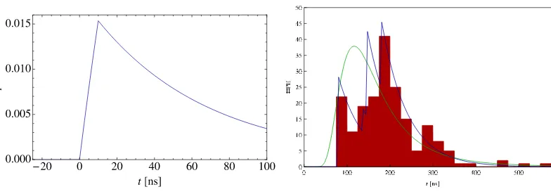
where the ideal unit response r(·) is given in Figure 1(a), the analytical expression being omitted for the sake of simplicity. Let the number Nμof muons crossing the tank be known. Adding the contributions of Nμmuons with signal amplitudes A=(A1, . . . ,ANμ) and arrival times t=(t1, . . . ,tNμ), the binwise
signal expectation is
¯ni(t,A)= Nμ
j=1
¯ni(tj,Aj).
Let now x=(t1,A1, . . . ,tNμ,ANμ). Our likelihood is finally
p(n|x)=
M
i=1
Poi¯ni(t,A)(ni). (4)
A summary of the generating model is depicted in Figure 1(b).
This model is only a sketch of what is needed to achieve inference in Auger: in practice, more nuisance variables have to be added, to describe, e.g., the noise in the detector electronics. Still, even with simple flat priors on x, integrals with respect to the resulting posterior
π(x)∝p(n|x)p(x)
cannot be analytically computed.
(a) The muonic time response model r(t). (b) An example signal
Figure 1. The generative model of the muonic signal. (a) Ideal unit response function r(·). (b) The green curve
is the time-of-arrival distribution p(tμ) used to generate this example with Nμ=4. The amplitude distribution is
not shown, but derives from the geometry of the tank. The blue curve is the ideal response4j=1Ajr(t−tj), and
the red histogram is the signal (PE count vector) n.
1.2 The Monte Carlo principle
Since integrals like (2) cannot be analytically derived, we have to rely on numerical approximation techniques. The cost of classical non-probabilistic numerical integration based on regular grids grows exponentially with the dimension d. The rationale behind Monte Carlo (MC) methods is to replace grids by stochastic samples. Let first
IN =
1 N
N
i=1
h(Xi). (5)
If X1, . . . ,XN∼πare independent and identically distributed (i.i.d.), then
IN ≈I=
h(x)π(x)dx. (6)
Note thatIn in (6) is a random variable. Its expectancy is precisely I (we say IN is an unbiased
estimator or I) and its variance is V/N, where V is the variance of h(X) when X∼π. This justifies the saying that Monte Carlo error decreases as √N.
Interestingly, one can see the MC principle as the randomization of a grid method: points are not regularly spread across the space anymore, but sampled according toπ. This is intuitively efficient, since regions of the space should be examined all the more finely that they contribute to the integral I. In other words, putting a fine grid whereπis large and a scarce one whereπis small will yield to an estimatorINwith small variance.
What makes a good MC method is thus its ability to sample fromπ. In this tutorial, we describe various ways of sampling according toπ, exactly or approximately. Note that the sampling methods we describe are generic and can find other, non-Bayesian applications in experimental physics: sim-ulators like CORSIKA [15] implement sampling from complex, hierarchized distributions with MC methods.
The rest of this tutorial is organized as follows. In Section 2 we review basic non-MC sampling methods and MC methods that are based on i.i.d. sampling. The latter are useful in small dimensions (say smaller than 10) and often require thatπcan be somehow approximated. Section 3 describes Markov chain Monte Carlo methods (MCMC). MCMC methods generate a dependent sample which asymptotically resembles a sample fromπ. Section 4 presents advanced MCMC tools that learn or exploit the structure ofπfor better sampling.
2 First sampling methods
2.1 The inverse cdf method
If the cumulative distribution function F ofπ is known and can be inverted, then it is enough to know how to sample U from a uniform distribution2on [0,1]. Indeed one can show that F−1(U) is then distributed according toπ. This can be applied to generate exponential variables, for example. However, this method is not applicable beyond simple distributions, since we usually cannot even compute F, as it requires integrating with respect toπ.
2.2 The transformation method
It is sometimes possible to obtain samples from X∼πby applying a transformation to variables Y that are easier to sample. For example, building on the exponential generator of Section 2.1, we can add two independent exponential variables with parameter 1 to obtain a Gamma variable with parameters (2,1), as is easily proven by a convolution. Again, this method is limited in its applications to simple distributions.
2.3 Rejection sampling
Rejection sampling is one of the simplest MC algorithms. It requires the knowledge of a distribution q onXwhich is easy to sample from, such as a Gaussian or a Gamma distribution, and a constant M>0 such that
π≤Mq. (7)
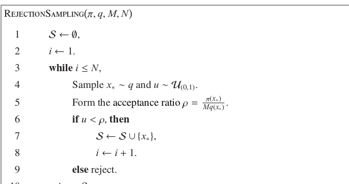
It works by repeatedly sampling according to a proposal distribution q and accepting or rejecting each sample with a certain probability that guarantees that the final accepted samples are distributed according toπ. The algorithm is presented in Figure 2.
Note that the tighter the bound in the right-hand side of (7), the less samples are rejected. Thus, a good knowledge of q and M is necessary for rejection sampling to be efficient. When such a bound is not known, one can resort to importance sampling.
2.4 Importance sampling
Importance sampling takes as input a proposal q but does not require (7), only that q puts mass wher-everπdoes. Furthermore, it only requires thatπis known up to a normalization constant. For clarity, we denote byπ0 the available unnormalized version ofπ, and will writeπonly for the normalized target distribution.
2We shall assume here that a uniform generator is available, the good old rand() function. However, implementing such a
RejectionSamplingπ,q,M,N
1 S ← ∅,
2 i←1.
3 while i≤N,
4 Sample x∗∼q and u∼ U(0,1).
5 Form theacceptance ratioρ= π(x∗)
Mq(x∗). 6 if u< ρ, then
7 S ← S ∪ {x∗},
8 i←i+1.
9 else reject.
10 returnS.
Figure 2. The pseudocode of the rejection sampling algorithm. The number of iterations to reach N samples
fromπis unknown beforehand and depends on the tightness of the bound in (7).
Unlike other algorithms in this chapter, each of which yields a sampleS, importance sampling return a weighted sample or, equivalently, an approximation of the target as weighted sum of point masses. Importance sampling is based on the law of large numbers [13, Section 7.5] with a reweight-ing trick. Precisely, importance samplreweight-ing approximates the integral I of (6) with the estimator
IN =
1 Z
N
i=1
wih(xi),
where
wi=
π0(xi)
q(xi)
, and Z=
N
j=1
wj. (8)
In general, the estimatorIN is not unbiased, but only asymptotically unbiased. Indeed, applying the
law of large numbers to both the numerator and the denominator, we obtain
IN=
N
i=1wih(xi)
N j=1wj
→
h(x)π0(x)dx
π0(x)dx =
h(x)π(x)dx, xi∼q i.i.d.
where the convergence is almost sure3. Note, however, that ifπ
0 =πis normalized, one can replace Z by N in (8) and obtain an unbiased estimator IN. The pseudocode of the importance sampling
algorithm is given in Figure 3.
To understand the rôle of the proposal q, it is useful to derive the asymptotic behaviour of the variance of the estimator:
Var(IN)=
σ2 lim N +o
1 N
, (9)
with
σ2 lim=
[h(x)−I]2π(x) q(x)π(x)dx.
Thus, in order to keep the variance of IN – in physical terms the square of the statistical error –
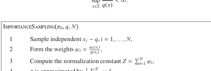
low, q has to be chosen close toπ, and with heavier tails thanπ. The last requirement means that we must ensure that
sup
x∈X
π(x) q(x) <∞.
ImportanceSamplingπ0,q,N
1 Sample independent xi∼q,i=1, . . . ,N,
2 Form the weightswi=πq(xi0(xi)),
3 Compute the normalization constant Z=iN=1wi,
4 πis approximated by Z1Ni=1wiδxi.
Figure 3. The pseudocode of the importance sampling algorithm only requires thatπis known up to a normal-ization constant. Unlike rejection sampling, no sample is wasted.
2.4.1 On the choice of the proposal for importance sampling
In practice, either a reasonable choice for q is available, or not. The first case occurs when, e.g.,π is almost unimodal and concentrates its mass on a small region ofX. A Gaussian centered at this small region with a reasonable variance then yields a good choice for q. Easy-to-sample, heavy-tailed distributions like Student’s distribution, are also handy. We have often seen the case in particle physics whereπis a posterior that puts all its mass on a small region ofRd. In that case, remember
that importance sampling with the right q yields better accuracy than grid-based methods or uniform sampling.
If the choice of q is not obvious, we recommend the use of an adaptive strategy, such as population Monte Carlo. A description of population MC and an application to model selection in cosmology can be found in [24]. Basically, first make a wild guess q(0)for q, say a Gaussian with a large variance. Apply importance sampling a first time to obtain an estimate of πand fit a Gaussian q(1) to this estimate ofπ. Now re-apply importance sampling with q(1)as a proposal, and re-fit a new Gaussian q(2)toπ, etc. After T iterations, q(T )should be a good proposal distribution for importance sampling. Of course, you can apply this procedure with other candidate proposals than Gaussians, you should indeed choose a family of distributions among which you think you may find a good approximation of
π. If you have reasons to believe thatπis bimodal, for example, you should probably fit a mixture of two distributions as in [24] rather than a Gaussian, which is unimodal. Usually, with the right choice of family of distributions, a few iterations are enough to get a reasonable q, and you can stop when q(t)does not change a lot with t.
2.4.2 Convergence diagnostics and confidence intervals
There are a variety of criteria to assess the good behaviour of an importance sampling estimator. An important thing to check is the empirical distribution of the weightswi. If only a few of the weights are
nonzero, the estimatorIN is based on too few points and thus has a large variance. It is thus desirable
to obtain a weight distribution with a high number of large and comparable weights, which, again, is achieved by finding a good proposal q.
More formal quality measures also exist, such as the so-called effective sample-size ESSN:
ESSN =
⎛ ⎜⎜⎜⎜⎜ ⎜⎝
N
i=1 ⎛ ⎜⎜⎜⎜⎜ ⎝Nwi
j=1wj
⎞ ⎟⎟⎟⎟⎟ ⎠ 2⎞ ⎟⎟⎟⎟⎟ ⎟⎠ −1 .
ESSNranges from 1 (when only one weight is nonzero) to N (when all weights are equal). Roughly,
ESSNis telling how many of the samples x1, . . . ,xNare really independent in the following sense: the
accuracy ofINis equivalent to the accuracy obtained with ESSNsamples that would be drawn directly
from the realπ.
Finally, it is possible to derive asymptotic confidence intervals forIN−I, since it can be first shown
that √
N(IN−I)→ N(0, σ2lim),
where the convergence is in distribution, and second
N
N
i=1 ⎛ ⎜⎜⎜⎜⎜ ⎝Nwi
j=1wj
⎞ ⎟⎟⎟⎟⎟ ⎠
2⎛ ⎜⎜⎜⎜⎜ ⎝h(Xi)−
N
k=1
wk
N j=1wj
h(Xk)
⎞ ⎟⎟⎟⎟⎟ ⎠ 2
→σ2 lim
almost surely.
2.5 Going to higher dimensions
We now consider an insightful example on how rejection and importance sampling scale when the dimension d of the ambient space grows. Consider a simple unit Gaussian target π = N(0,Id),
where Id is the d×d identity matrix. Say we are fortunate enough to know thatπis an isotropic
Gaussian, but ignore its variance. A relevant choice of proposal would then be an isotropic Gaussian q(x)=N(0, σ2I
d).
If applying rejection sampling, one must know beforehand thatπhas variance upper bounded by some constantσ∗, and then chooseσ ≥ σ∗, in order to satisfy (7). This is already a very strong assumption, but there is worse: the fraction of accepted samples goes asσ−d. This means that ifσis
not exactly 1, one should expect an exponentially small number of accepted samples with growing d. A similar curse of dimensionality happens with importance sampling: the variance of the weights is either infinite ifσ≤ √1
2, or it goes asσ
d.
2.6 Conclusion on rejection and importance sampling
3 MCMC basics
Rejection and importance sampling are Monte Carlo methods based on an i.i.d. sample from a pro-posal distribution q. To tackle large dimensions, other methods have been devised that are based on a non-independent sampling: Markov chain Monte Carlo methods (MCMC). The prototype of MCMC methods is the Metropolis-Hastings algorithm, of which almost all MCMC algorithms are variants. Note that although we concentrate here on applications to inference, MCMC is also used in simulators like CORSIKA, see [8] for an example.
3.1 The Metropolis-Hastings algorithm
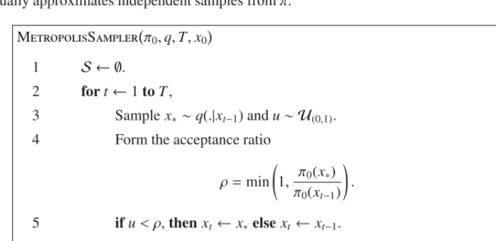
We first describe Metropolis’ algorithm in Figure 4. It builds a random walk (Xi) that exploresX, and
eventually approximates independent samples fromπ.
MetropolisSamplerπ0,q,T,x0
1 S ← ∅.
2 for t←1 to T ,
3 Sample x∗∼q(.|xt−1) and u∼ U(0,1).
4 Form the acceptance ratio
ρ=min
1, π0(x∗)
π0(xt−1)
.
5 if u< ρ, then xt←x∗else xt ←xt−1.
6 S ← S ∪ {xt}.
7 returnS.
Figure 4. The pseudocode of the Metropolis algorithm.
Metropolis’ algorithm is a for loop. At each iteration t, a candidate point x∗ is proposed in the neighborhood of the current position xt−1, according to a proposal q(·|xt−1). In Metropolis’ algorithm, this proposal is assumed to be symmetric, i.e., q(x|y) = q(y|x). In practice, a Gaussian with fixed covariance matrixΣis often used: q(y|x)=N(y|x,Σ). After the candidate point has been generated, it is accepted as the next position xtonly with a certain probabilityρ, which is 1 ifπ(x∗) is larger than
π(xt−1), and smaller than 1 (but often not zero!) if not. This precise definition ofρrelates the random
walk (Xi) toπand makes the algorithm different from an optimization algorithm: it does not always
try to move for a point with largerπ. Furthermore, the theory of Markov chains4guarantees that such an acceptance rule implies thatπis the limiting distribution of the chain (Xi), in a sense that shall
become clear soon.
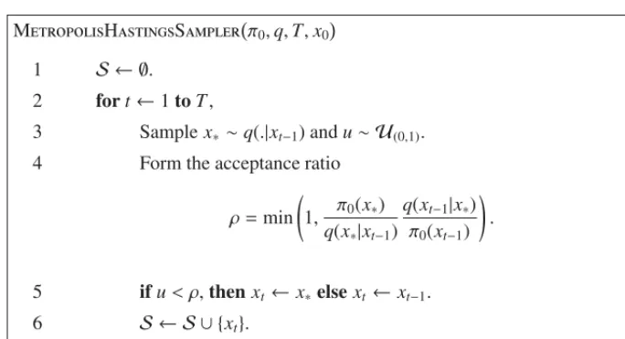
Now we are ready to present the Metropolis-Hastings (MH) algorithm. It is simply Metropolis’ algorithm, but with general, possibly nonsymmetric proposals. The pseudocode of MH is given in Figure 5. Note the new definition of the acceptance probabilityρ, which ensures the final convergence toπ. Intuitively, this acceptance rule cancels the influence of q on the limiting distribution: the probability of accepting a move that q is likely to draw often is reduced.
4A Markov chain is a sequence of random variables (X
i) such that Xi+1depends on the past only through Xi. More formally:
MetropolisHastingsSamplerπ0,q,T,x0
1 S ← ∅.
2 for t←1 to T ,
3 Sample x∗∼q(.|xt−1) and u∼ U(0,1).
4 Form the acceptance ratio
ρ=min
1, π0(x∗) q(x∗|xt−1)
q(xt−1|x∗)
π0(xt−1)
.
5 if u< ρ, then xt←x∗else xt ←xt−1.
6 S ← S ∪ {xt}.
7 returnS.
Figure 5. The pseudocode of the Metropolis-Hastings algorithm.
We refer the reader interested by a gentle introduction to theoretical results on MH to [18, Chapter 7]. We will limit ourselves to one simple but useful result, since it covers the common Metropolis algorithm with Gaussian proposals: assume q(·|x) puts mass over allXand that there existsδ >0 and
ε >0 such that
x−y< δ⇒q(y|x)> ε,
then for any integrable function h, MH gives an asymptotically unbiased estimate of the integral I defined in (6):
lim
N→∞IN→I.
This is an example of formal result that states that (Xi) behaves like independent draws fromπfor
large i.
3.2 Assessing convergence
MH outputs a sample from a Markov chain that asymptotically approximates independent draws from
π. From a practitioner’s point of view, two questions arise, which we address successively in the rest of this section. First, since we are waiting for the chain (Xi) to converge toπwhatever starting value
x0we input, it is important to know from which iteration on the chain is independent from x0. Second, even if the iteration number is big enough that the chain has “forgotten” about x0, a Markov chain is not a series of independent draws, and it is relevant to ask whether our MCMC chain has reached a good approximation of independence, or, in other words, how much the variance of the estimator IN
suffers from the statistical dependence among the Xis.
3.2.1 Has the chain forgotten its starting state?
many chains with different starting points, and check they all give similar results. Besides traceplots, one can plot an online estimate of the mean:
1 n
n
i=0 Xi
versus n=1, . . . ,N for all chains and check they all converge towards the same value. If not, then con-vergence has certainly not been reached. Online estimates of the variance of each chain, of quantiles, etc. can also be useful to plot. There are a number of statistics of the sample that formalize this prin-ciple of comparison between many chains. A popular such convergence assessment is known as the Gelman-Rubin diagnosis [18, Section 12.3.4]. See [18, Chapter 12] for a review of other convergence diagnostics.
To cancel the influence of the starting point in the evaluation ofIN, it is usually advised to discard
the first B samples of the chain and replaceINby
IN,B=
1 N−B+1
N
i=B
Xi.
The discarded B samples are called a burn-in sample. Though reducing initialization bias, discarding the first B samples also usually makes the variance ofIN,B larger than the variance ofIN, and so B
should be as small as possible to keep the final statistical error low. The choice of an optimal B is an open question. In practice, our personal take is to keep the burn-in below 25% of the sample, and simply go for a large enough number of samples N that multiple chains with different initializations give similar answers.
3.2.2 How independent do the samples look?
After initialization bias, the second convergence issue is that of the independence of the samples. Identifying an MCMC chain converging toπto a dynamical system progressively stabilizing at equi-librium, Sokal speaks here of autocorrelation in equilibrium [23]. This is related to the variance of IN
in the following way: the more correlation there is between samples (Xi) (the autocorrelation of the
chain), the higher the variance ofIN. The variance ofINwill still decrease in K/N, but the constant K
might be much larger than in the independent case [23].
Again, theoretical answers to this question are not very satisfying as of today, but practical di-agnostics exist. Besides plotting the different components of the chain (Xi) versus i and checking
independence, the simplest idea is to plot the autocorrelation function of the chain. If d = 1, it is defined as
ρ(t)= C(t)
C(0), where C(t)= 1 N−t+1
N−t
i=0
(Xi−X)(Xi+t−X), (10)
where X=N−1Ni=1Xi. If d>1 one considers the autocorrelation in each component. The
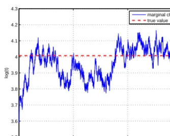
autocor-relation function for t ≥0 should look like a rapidly decreasing exponential starting at 1 and going to 0, as in Figure 7(b). If not, then one can thin the chain, i.e., keep only one sample every other 10 or higher if necessary. But while this may lead to more independent samples, it also leads to a waste of computational effort and an increase in the variance of the final estimator. If strong autocor-relation is revealed, we recommend to start all over with a different q. Indeed, strong autocorrelation often reveals a bad choice in the proposal. Finally, note that if one is only interested in estimating
3.2.3 Tuning the proposal distribution of MH
Consider the Metropolis algorithm of Figure 4. If q proposes only small steps, then the candidates x∗ will often be accepted since the ratio of the posteriors in Step 4 of Figure 5 will be close to 1. This will lead to high acceptance but also high autocorrelation: Xi+1is almost always in the neighborhood of Xi, and the chain needs a lot of iterations to cross the space, see Figure 6(a) for a typical traceplot. On
the other hand, if q proposes too big steps, then it is likely that they will be rejected, especially if the current state of the chain has a high value ofπ. This will lead to the chain being blocked for several iterations, which is an even worse case of autocorrelation, see Figure 6(b) for a typical traceplot. There is thus a compromise to find between small steps and large acceptance rate, and large steps and small acceptance rate. Theory suggests that when the target and the proposals are Gaussian, the acceptance rate to reach minimum variance ofINis approximately 0.5 when d ≤2 and 0.25 otherwise [19, 20].
In the common case where the proposal is Gaussian, practitioners usually proceed as follows: take a proposal with some free stepsize parameterσ:
q(y|x)=N(y|x, σΣ0), (11)
launch several preliminary runs with different values for σ, and finally select the value of σ that yielded the desired acceptance rate for the final run.
At this stage, we personally advocate the use of a pseudoadaptive strategy: adaptive because it learns a goodσalong the run, and pseudo because we stop the adaptation before the end of the burn-in5. While t≤B, where Bis smaller than the burn-in length B, we advise to adaptσin the following manner: at each iteration t, replace log(σ) by
log(σ)+ 1 t0.7(αt−α
∗) (12)
whereαt ∈ [0,1] is the current acceptance rate (the number of accepted samples so far divided by
t),α∗ is 0.5 if d≤2 and 0.25 else. The log transformation guarantees thatσremains positive. The rationale behind (12) is that ifαt > α∗, then too many steps are accepted, so that the stepsize should
be increased, and vice versa. (12) with a large enough Bis simply an automatic way to perform the preliminary search forσ.
3.2.4 Asymptotic confidence intervals forIN
After having obtained a sample with good properties as discussed previously, we are interested in deriving a confidence interval forIN−I. Note that this is not the same as finding a credible interval
as in Figure 7(d): we are here interested in knowing howINvaries when the full sample (X1, ...,XN)
varies, being drawn from the same chain. It is a tougher and more open question than with importance sampling. First, we need to check that the chain satisfies a central limit theorem (CLT):
√N(
IN−I)→ N(0, σ2lim)
where the convergence is in distribution. A discussion on the CLT for Markov chains can be found in [18, Section 6.7.2], with a note on MH in [18, Section 7.8.2]. For our needs, we just state that a CLT holds for Metropolis’ algorithm with Gaussian proposals and a target with bounded support, see [16, Theorem 4.1]. Now, when a CLT holds, confidence intervals can be built using proper6 approxima-tions ofσ2
lim [10]. These estimators ofσ2limare not difficult to understand, but their description and 5In Section 4.1, we discuss a fully adaptive algorithm where a similar adaptation is carried out to the end of the run. 6By proper, we mean a sequenceσNthat converges toσ
the conditions for convergence are fairly technical, and we refer the interested reader to [Theorems 1 and 2][10] for recent results on the so-called spectral and overlapping batch means method, our two favourites. A less technical but not up-to-date spectral method is described in [23, Section 3].
3.3 Implementation tips
First, MCMC can deal with constrained variables. If the variable is discrete, it is usually easy to find a proposal with the right constrained support. Constrained continuous variables are to be treated differently. One could, for example, include an indicator in the prior that will yield rejection of all points outside the allowed region. But ifπis large near the boundary of this allowed region, it is likely that the chain will spend time there and thus a lot of points will be rejected only because they do not satisfy the constraint. This is a waste of computational effort, and, if possible, it is usually advised to reparametrize the problem so that it becomes unbounded. If x has to remain positive, then use log(x). If x has to remain in an interval, then use Argth, for example.
Second, as with most multivariate methods, it is usually better to scale one’s variables. The rough idea is that a step in every direction should have the same effect onπ. This should make Gaussians with covariance proportional to the identity reasonable proposals.
Third, whenever manipulating likelihoods, it is advisable to work in the log domain. Comput-ing log-likelihoods is numerically more stable than doComput-ing large products of potentially very small numbers, and MCMC code can always be written using only log-likelihoods.
3.4 A worked out example
Consider the model of Section 1.1 with a single muon entering the tank: Nμ=1. We simulated data with an arrival time ttrue = 55 and an amplitude Atrue = 20. The simulated signal n is depicted in Figure 7(a).
We place a wide independent Gaussian prior on t and A: p(t,A)= N(t|100,1002)N(A|20,202). Let us apply MH to obtain the posterior p(t,A|n). First, let us change variables for log(t) and log(A),
to avoid dealing with a boundary inR2. log(t) and log(A) roughly have the same scale, so we do not modify them further. Let T =20 000 iterations, of which we discard the first B=5 000 as burn-in. We take a Gaussian with covarianceσ2I as a proposal and apply the pseudoadaptive tuning of (12).
The results7 can be seen in Figures 7(a) to 7(e). The autocorrelation function in Figure 7(b) indicates a fairly independent behaviour of the chain. This is confirmed by the traceplot in Figure 7(c) where no clear dependence can be detected by eye.
To obtain marginal distributions ofπ, one can simply collect the corresponding coordinate among the Xis. The marginal histograms here look regular, as shown by the log(t) marginal in Figure 7(d).
The acceptance has approximately reached the optimal 50% by the end of the burn-in and stabilized there. To check independence from the starting point, we ran 10 chains with uniform initialization on a wide rectangle, and plotted the online sample mean and standard deviations of each chain in Figure 7(f): all chains are consistent.
When reporting a result, the best practice is to give a summary of and make available the entire posterior sample. WhenXis high-dimensional, a series of marginal histograms, or 2D plots of one component versus the other, etc. can be given. In terms of estimation, credible intervals with level c can be computed easily once the sample has been drawn: simply report any interval that contains a proportion c of the samples. Such an interval is computed and given in Figure 7(d), for example.
0.5 1 1.5 2 x 10⁴
3.5 3.6 3.7 3.8 3.9 4 4.1 4.2 4.3
iteration number
log(t)
marginal chain true value
(a) Steps too small, acceptance too high
0.5 1 1.5 2 x 10⁴
2.6 2.8 3 3.2 3.4 3.6 3.8 4 4.2 4.4 4.6
iteration number
log(t)
marginal chain true value
(b) Steps too big, acceptance too low
Figure 6. Two examples high autocorrelation with different causes.
Finally, we give here two highly correlated traceplot examples of badly tuned chains that should ring an alarm, and be compared to the correct behaviour in Figure 7(c). On Figure 6(a),σis too small, leading to an overly slow exploration of the parameter space. On Figure 6(b),σis too large, causing the chain to stay blocked very often.
3.5 Physics-inspired variants of MH: Gibbs, Langevin and Hamilton
MH with a simple unimodal proposal (Gaussian, Student) is very generally applicable, but can be enhanced through the use of additional information on the target distributionπ. Although, in our experience, they are rarely used in experimental physics due to the complexity of the models, we quickly review here some popular variants of MH that were actually inspired by physics.
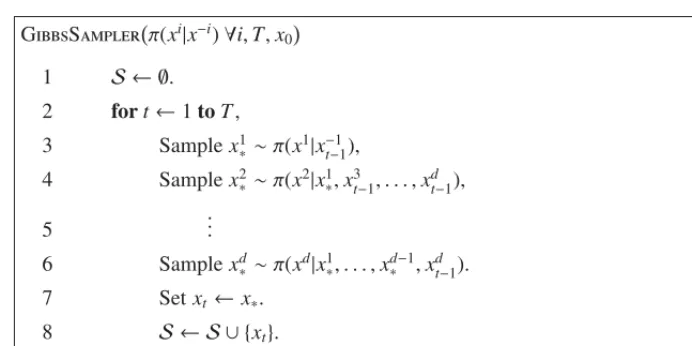
3.5.1 The Gibbs sampler
For x=(x1, . . . ,xd)∈Xa vector8of length d, define x−i=(x1, . . . ,xi−1,xi+1, . . .xd). If the posterior
is simple enough that it is easy to sample from all conditional distributionsπ(xi|x−i), then one can
replace Step 3 of MH in Figure 5 by a sequence of draws from the conditionals, conditioning on the components already drawn. The acceptance probabilityρin Step 4 in Figure 5 then evaluates to 1 and every proposal is thus accepted. The pseudocode of the Gibbs sampler is given in Figure 8.
The Gibbs sampler is useful in models where the dependencies between variables are non-trivial, but the conditional distributions are easy to sample. Even if this is rarely the case in particle physics, it can happen that some conditional distributions are available, and one might then use Gibbs proposals on some of the variables within an MH scheme. Any concatenation of MCMC steps is permitted, as long as the same concatenation is repeated over and over.
3.5.2 Langevin diffusion
If not the conditionals, one might know how to compute the gradient ofπ. This is also useful informa-tion: although MH is not an optimization algorithm, visiting all modes ofπis essential. The Langevin
0 50 100 150 200 250 300 350 0 0.5 1 1.5 2 2.5 3 3.5 4 4.5 5
# of PEs
t [ns]
(a) Generated signal
0 5 10 15 20 25 30 −0.2 0 0.2 0.4 0.6 0.8 Lag Sample Autocorrelation
(b) Autocorrelation function
0.5 1 1.5 2 x 10⁴
3.4 3.6 3.8 4 4.2 4.4 4.6 4.8 5 iteration number log(t) marginal chain true value
(c) log(t) chain
3.4 3.6 3.8 4 4.2 4.4 4.6 4.8 5 0 500 1000 1500 2000 2500 3000 3500 4000 log(t)
# of occurrences
marginal histogram true value marginal mean 95% credible interval
(d) log(t) histogram
0 0.2 0.4 0.6 0.8 1 1.2 1.4 1.6 1.8 2 x 10⁴
0 0.1 0.2 0.3 0.4 0.5 0.6 0.7 0.8 0.9 1 iteration number acceptance (e) Acceptance
0 0.2 0.4 0.6 0.8 1 1.2 1.4 1.6 1.8 2 x 10⁴
−1 0 1 2 3 4 5 6 7 8 iteration number log(t) true value online mean online mean +/− 3 online std
(f) Statistics of 10 independent chains
GibbsSamplerπ(xi|x−i)∀i,T,x0
1 S ← ∅.
2 for t←1 to T ,
3 Sample x1
∗∼π(x1|x−t−11),
4 Sample x2
∗∼π(x2|x∗1,x3t−1, . . . ,x
d t−1),
5 ...
6 Sample xd
∗ ∼π(xd|x1∗, . . . ,x∗d−1,xdt−1). 7 Set xt← x∗.
8 S ← S ∪ {xt}.
9 returnS
Figure 8. The pseudocode of the Gibbs sampler.
sampler is an MH sampler with a proposal that is partly deterministic: from xt−1, a small step in
the direction of the gradient ofπat xt−1 is done, and from there a small Gaussian step is performed. Basically, the Langevin sampler is MH with proposal
q(y|x)=N(y|x+σ 2
2 ∇logπ(x), σ 2I
d).
The Langevin sampler is actually inspired by the discretization of a diffusion equation [18, Section 7.8.5 and references therein]. Interestingly, the MH acceptance step can here be interpreted as a correction for the discretization error of the numerical scheme solving the diffusion equation.
Another popular sampler, inspired by mechanics, is Hamiltonian MCMC, or hybrid MCMC [17]. Its main features are that the target is plugged in an energy function, points in Xare interpreted as space coordinates and augmented with an artificial momentum variable, and proposals include a deterministic move along an approximate solution to a system of differential equations, as well as an MH correction step. Hamiltonian MCMC in its original form also requires a closed form for the gradient, which is again rarely available. Details of the pseudocode of Hamiltonian MCMC are out of the scope of this chapter, but we refer interested readers to [17].
4 Advanced MCMC methods
(4) is invariant to the ordering of the muons. This has undesirable effects on marginal inference that MCMC can cope with, as presented in Section 4.2.
4.1 Adaptive MCMC
We already mentioned a pseudoadaptive update scheme in (12), where the stepsize of the MH proposal was tuned during a finite number of iterations before being frozen for the rest of the run. Now a legitimate question is whether the asymptotic guarantees on MCMC hold if we let the adaptation run forever?
Adaptive MCMC is a research topic that focuses on designing provably valid MCMC algorithms with proposals that are tuned on the fly until the complete end of the run. The literature is dense, and we single out here one adaptive MCMC algorithm that we use in almost every physics application: the adaptive Metropolis algorithm (AM; [14]).
The pseudocode of AM is given in Figure 9. Note that in practice, it may help to wait for say 10d iterations before using the adapted covariance matrix in the proposal. βshould be taken in (12,1], 1 meaning freezing the covarianceΣt faster. By default, we personally use 0.7. In the literature, the
covariance matrix scale factor, or stepsize,σis often set to (2.38)2/d, as it is shown in [19] that this stepsize is optimal in a sense for Gaussian proposals and targets. However, in practice, we recommend the use of an adaptive scheme such as Step 9 in Figure 9, which preserves the convergence of AM. Other adaptive scalings are discussed in [2].
Remark that AM is still called an MCMC algorithm, although the chain is not Markov anymore: given Xt−1, Xt is still dependent on the previous history of the chain throughΣt−1. Still, AM was
proven to provide an asymptotically unbiased estimatorIN [1].
AdaptiveMetropolisSamplerπ0,μ0,Σ0,β∈(12,1],σ0,T,x0
1 S ← ∅.
2 for t←1 to T ,
3 Sample x∗∼ N(.|xt−1, σt−1Σt−1) and u∼ U(0,1).
4 Form the acceptance ratio
ρ=min
1, π0(x∗)
π0(xt−1)
.
5 if u< ρ, then xt←x∗else xt ←xt−1.
6 S ← S ∪ {xt}.
7 μt←μt−1+t1β
Xt−μt−1
8 Σt←Σt−1+t1β
(Xt−μt−1) (Xt−μt−1)T−Σt−1
9 log(σt)←log(σt−1)+t1β(ρ−α∗)
10 returnS.
Figure 9. The pseudocode of the adaptive Metropolis algorithm. Modifications with respect to the Metropolis
algorithm in Figure 4 are Steps 7 to 9 (in blue). The setting of free parametersβand c is discussed in the main
4.2 Label switching
Another feature of the likelihood (4) is that it is invariant to permutations of the muons. In the case where Nμ=2, for example,
p(n|t1,A1,t2,A2)=p(n|t2,A2,t1,A1).
If the prior is also invariant, then the posteriorπ inherits the same property. πhas then as many redundant modes as there are permutations to which it is invariant, and this is undesirable when it comes to marginal inference. Indeed, Figures 10(a) and 10(b) illustrate the challenges when running vanilla AM on the example presented in Figure 7(a). The red variable gets stuck in one of the mixture components, whereas the blue, green, and brown variables visit all the three remaining components, a phenomenon called label switching. As a result, marginal estimates computed for the blue, green, and brown variables are then mostly identical as seen on Figure 10(b). In addition, the shaded ellipses, depicting the marginal posterior covariances of the two parameters t and A of each muon, indicate that the resulting empirical covariance estimate is very broad, resulting in poor efficiency of the adap-tive algorithm. Label switching is addressed by so-called relabeling algorithms [5, Chapter 8]. A recent relabeling mechanism that interweaves favorably with AM can be found in [6], along with an application to the Auger model of Section 1.1.
4.3 Transdimensional problems
Until now, we have always considered Nμ fixed and known. Now consider the problem of letting Nμfree and trying to estimate it. This problem is termed model selection in statistics, and various Bayesian answers have been given. One full MCMC solution is called reversible jump MCMC (RJM-CMC) and is due to Green [12]. We will introduce the algorithm through an example here, the generic description of the method and implementation advice can be found in [18, Section 11.2].
Say we know there were 1≤Nμ ≤2 muons in the tank from some other measurements, and we would like to infer Nμas well as the corresponding times and amplitudes. Let the prior on Nμbe
p(Nμ=1)=p(Nμ=2)=1 2.
We need a chain that targets
π(x)∝p(n|Nμ,t1,A1, . . . ,tNμ,ANμ)p(t1,A1, . . . ,tNμ,ANμ|Nμ)p(Nμ)
and that can take values such as (1,t,A) and (2,t1,A1,t2,A2). In other words, the state space of the chain would be
{1} ×R2∪ {2} ×R4.
This chain should be able to jump within models, i.e., from (1,t,A) to (1,t,A) or from (2,t1,A1,t2,A2) to some other point (2,t1,A1,t2,A2) with two muons. The chain should also be able to jump across models, i.e., from (1,t,A) to some point (2,t1,A1,t2,A2) and vice versa. For jumps within the same model, we implement usual MH moves. The main contribution of RJMCMC is a general rule to build jumps across models and the corresponding acceptance probability. The key is to design jumps across models that are likely to be accepted. In our example, to jump from a point (Nμ= 1,t,A) to (Nμ=2,t1,t2,A1,A2), we may break a muon into two separate muons with roughly half the original amplitude each:
(a) AM: component chains and means
(b) AM: component posteriors
Figure 10. The results of AM on the signal example of Figure 1(b). (a) Three of the four t chains switch position
constantly as a result of the targetπbeing invariant to permutations of the muons. The corresponding running
means (thick lines) converge to similar values. For reference, the thick black line depicts the mean of the coloured thick lines. (b) Label switching causes artificially multimodal marginals. Black dots: the x-coordinates are the
real time-of-arrival parameters t, and they-coordinates are proportional to the amplitudes A. Colored ellipses are
exp(1/2)-level sets of Gaussian distributions: the means are the Bayesian estimates of (t,A) for each muon, and
the covariance is the marginal posterior covariance of each (t,A) couple.
This move can be summarized by the application of a one-to-one transformation
T1→2(t,A,u, v)=(t−u, A
2 −v,t+u, A 2 +v),
whose jacobian is J1→2 = 2. Now that this move from a model with one muon to a model with two muons is fixed, the opposite move is constrained in RJMCMC. A valid choice is the inverse transformation T−1, with Jacobian J
2→1 =1/2. Finally, the user has to specify the probabilities p1→2 and p2→1 that a move from Nμ =1 to Nμ=2 is proposed and vice versa. In the end, the acceptance probabilityρof a move from (1,t,A) to (2,t1,A1,t2,A2) is given by
ρ=min ⎛ ⎜⎜⎜⎜⎜
⎝1,J1→2 π
(2,t1,A1,t2,A2)
π(1,t,A)q(t2−t1 2 )r(
A2−A1 2 )
p2→1 p1→2 ⎞ ⎟⎟⎟⎟⎟ ⎠,
and the acceptance probabilityρof a move from (2,t1,A1,t2,A2) to (1,t,A) is given by
ρ=min ⎛ ⎜⎜⎜⎜⎜ ⎝1,J2→1
π(1,t,A)q(t2−t1 2 )r(
A2−A1 2 )
π(2,t1,A1,t2,A2)
p1→2 p2→1 ⎞ ⎟⎟⎟⎟⎟ ⎠.
RJMCMC is very generic, but transdimensional moves have to be designed with care to be ac-cepted often enough. However, once the chain obtained, inference on Nμis as easy as on any other parameter: simply count how many times Nμ =1 in the chain, divide it by the length of the chain, and you have the posterior probability that Nμ=1 ! Reporting the results of an RJMCMC chain can be tricky. Here, one could report the posterior distribution on Nμ, and plot the marginals of the other parameters for the most probable values of Nμ. Sophisticated summaries have recently been proposed [21], which can compute the probability that one muon in particular is present. Finally, we note that while AM and relabeling can be merged, further including reversible jumps is still research work.
5 Conclusion and the Monte Carlo ladder
We reviewed basic Monte Carlo ideas and methods, along with some advanced ones like adaptive MCMC. We tried to give intuition for picking the right method, since none is uniformly powerful, and practical advice on implementations. To sum up the algorithms presented here and point to other important ones that we did not cover, we adapt and complete Murray’s integration ladder9. Growing item number meanshigher practical complexity, but also eitherhigher efficiencyorwider applicability. Check [18] when no further reference is given.
1. Quadrature,
2. Rejection sampling,
3. Quasi-MC,Importance sampling,
4. MCMC(MH, slice sampling, etc.),
5. Adaptive MCMC[4],hybrid MC [17], tempering methods[11], sequential MC [7], particle MCMC [3].
6. Approximate Bayesian computation (ABC; [9]).
6 Appendix: Notations, acronyms, and recommended readings
Target densities.πalways denotes the target probability density function, which in Bayesian inference problems is a posterior. Its support isX ⊂Rd, and so d denotes the dimension of the problem. π
0 denotes an unnormalized version ofπ, formally written asπ0 ∝π. In Bayesian inference problems,
π0is often of the form likelihood×prior.
Estimators. IN always denote the estimator defined in (5), but the Xis used to build it depend on
the context.INonly denotes the importance sampling estimator.
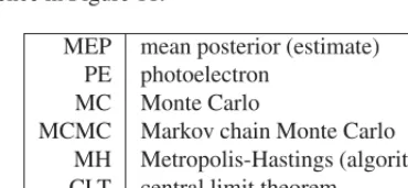
Distributions. We write X ∼ p when the probability density function of X is p. Used acronyms are summed up for reference in Figure 11.
MEP mean posterior (estimate) PE photoelectron
MC Monte Carlo
MCMC Markov chain Monte Carlo MH Metropolis-Hastings (algorithm) CLT central limit theorem
AM adaptive Metropolis (algorithm)
Figure 11. Glossary of acronyms, in order of appearance.
For further reading on MC methods, we strongly recommend the textbook [18], to which this tutorial owes a lot. We have tried to refer to specific parts of this book whenever possible. An introduction to MCMC specifically meant for physicists is [23]. While it is a bit outdated now, it still provides insightful and untraditional explanations, especially on assessing MCMC convergence.
Acknowledgments
I would like to thank the SOS organizers for inviting me to lecture, and for proposing a rich cross-disciplinary programme that generated many interesting discussions. A large part of this tutorial was written while I was working in the Auger group at LAL, Orsay (France).
References
[1] C. Andrieu, E. Moulines, and P. Priouret. Stability of stochastic approximation under verifiable conditions. SIAM Journal on Control and Optimization, 44:283–312, 2005.
[2] C. Andrieu and J. Thoms. A tutorial on adaptive MCMC. Statistics and Computing, 18:343–373, 2008.
[3] Christophe Andrieu, Arnaud Doucet, and Roman Holenstein. Particle Markov chain Monte Carlo methods. Journal of the Royal Statistical Society B, 2010.
[4] Y. Atchadé, G. Fort, E. Moulines, and P. Priouret. Bayesian Time Series Models, chapter Adaptive Markov chain Monte Carlo: Theory and Methods, pages 33–53. Cambridge Univ. Press, 2011. [5] R. Bardenet. Towards adaptive learning and inference – Applications to hyperparameter tuning
and astroparticle physics. PhD thesis, Université Paris-Sud, 2012.
[8] H. J. Drescher, M. Hladik, S. Ostapchenko, T. Pierog, and Werner K. Parton-based Gribov-Regge theory. Physics Reports, 2001.
[9] P. Fearnhead and D. Prangle. Constructing summary statistics for approximate Bayesian compu-tation: semi-automatic ABC. Journal of the Royal Statistical Society B, 2012.
[10] J. M. Flegal and G. L. Jones. Batch means and spectral variance estimators in Markov chain Monte Carlo. Annals of Statistics, 38(2):1034–1070, 2010.
[11] W.R. Gilks, S. Richardson, and D. Spiegelhalter, editors. Markov Chain Monte Carlo in Prac-tice. Chapman & Hall, 1996.
[12] P. J. Green. Reversible jump Markov chain Monte Carlo computation and Bayesian model determination. Biometrika, 82(4):711–732, 1995.
[13] G. R. Grimmett and D. R. Stirzaker. Probability and random processes. Oxford science publi-cations, second edition, 1992.
[14] H. Haario, E. Saksman, and J. Tamminen. An adaptive Metropolis algorithm. Bernoulli, 7:223– 242, 2001.
[15] D. Heck, J. Knapp, J. N. Capdevielle, G. Schatz, and T. Thouw. CORSIKA: A Monte Carlo code to simulate extensive air showers. Technical report, Forschungszentrum Karlsruhe, 1998. [16] S. F. Jarner and E. Hansen. Geometric ergodicity of Metropolis algorithms. Stochastic processes
and their applications, 341–361, 1998.
[17] R. M. Neal. Handbook of Markov Chain Monte Carlo, chapter MCMC using Hamiltonian dynamics. Chapman & Hall/CRC Press, 2010.
[18] C. P. Robert and G. Casella. Monte Carlo Statistical Methods. Springer-Verlag, New York, 2004.
[19] G. Roberts, A. Gelman, and W. Gilks. Weak convergence of optimal scaling of random walk Metropolis algorithms. The Annals of Applied Probability, 7:110–120, 1997.
[20] G. O. Roberts and J. S. Rosenthal. Optimal scaling for various Metropolis-Hastings algorithms. Statistical Science, 16:351–367, 2001.
[21] A. Roodaki. Signal decompositions using trans-dimensional Bayesian methods. PhD thesis, Supélec, 2012.
[22] D. S. Sivia and J. Skilling. Data Analysis: A Bayesian Tutorial. Oxford University press, second edition, 2006.
[23] A.D. Sokal. Monte Carlo methods in statistical mechanics: Foundations and new algorithms, 1996. Lecture notes at the Cargèse summer school.