DOI: 10.1051/epjconf/20134701007 C
Owned by the authors, published by EDP Sciences, 2013
Classification of variable stars in the WFCAM Transit Survey
Hristo Stoev
1,a, David Barrado
2,1, Luis M. Sarro
3and Andrés Moya
11Departamento de Astrofísica, Centro de Astrobiología (CSIC-INTA), PO Box 78,
28691 Villanueva de la Cañada, Spain
2Calar Alto Observatory, Centro Astronómico Hispano-Alemán, c/ Jesús Durbán Remón, 2-2,
04004 Almería, Spain
3Departamento de Inteligencia Artificial, Universidad Nacional de Educación a Distancia,
c/ Juan del Rosal, 16, 28040 Madrid, Spain
Abstract. The WFCAM Transit Survey is a photometric survey in the near-infrared and aims at finding
Earth-like planets transiting M-dwarf stars. As a by-product of the survey, a variety of variable stars has been detected. We report the discovery and classification of 192 periodic variable stars in the WFCAM Transit Survey. 185 of those objects are previously unknown variable sources. The derived parameters of their light curves will be helpful for the creation of a robust sample of light curves (and their parameters thereof) of classified variable stars in the near-infrared for the automatic classification of light curves of stellar objects in the J-band.
1. INTRODUCTION
The studies of variable stars have been one of the main fields of research in astronomy. In recent years, time-resolved photometric surveys have marked a memorable boom in time-domain astronomy. Projects such as OGLE, ASAS and Pan-STARRS are constantly monitoring the night sky from Earth and as a by-product, catalogs of variable stars are created. The space missions CoRoT and Kepler, dedicated to the search of transiting extrasolar planets and asteroseismology, have also produced detailed censuses of the variable star population in their fields. With the ongoing Vista Variables in the Vía Lactea (VVV) ESO Public Survey with an expected detection of∼106 variable point sources and the soon-to-be-launched Gaia spacecraft, which will monitor more than 109objects over the whole sky allowing the discovery of millions of variable stars [1], all those new detected variable sources will need to be properly classified.
2. THE WTS SURVEY
The WFCAM Transit Survey is an ongoing photometric survey campaign operating on the 3.8-m United Kingdom Infrared Telescope (UKIRT) since August 2007. The survey is monitoring 4 target fields, each of which covering 1.5 square degrees of sky, with the Wide-Field Camera imaging array in the infrared wavelengths (J-band, 1.25m) [2].
Each of the fields is observed by conducting eight pointings of the WFCAM pawprint. Then they are tiled together in order to provide a uniform coverage across the field. The cadence of the resulting light curves is 4 data points per hour. Depending on the weather conditions, the observations are usually carried out at the beginning of the night in>1” seeing when the atmosphere is still cooling and settling.
ae-mail:[email protected]
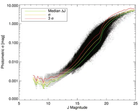
Figure 1. A graphical representation of the distribution of error as a function of the magnitude. The yellow line
represents the median error (J) for each 0.05-magnitude bin; the red line plots the standard deviation as a function of magnitude and the green line is the 3level of variation of the error with respect to the median error per bin.
Initial reduction of the raw images is performed using the Cambridge Astronomical Survey Unit (CASU) pipeline, based on the INT wide-field survey pipeline [3]. A so-called “master frame” is created by stacking the best 20 images based on their point-spread function (PSF). Source detection is performed on this image and then by means of aperture photometry, the brightness of each object detected on the master frame is measured on the rest of the frames and a catalogue is generated. At the end of the cycle, the data is written on quadruple-extension FITS binary table, i.e. one FITS container per detector.
The variable stars that are reported in this publication are all found in one of the WTS fields, approximately centered on the following coordinates:=19h35m,= +36◦30, hereafter referred to as the 19hr field.
3. DATA SET
3.1 Data Characterisation and Reduction of the WTS Light Curves
The 19hr field is the field with most extensive coverage and constitutes of 1145 epochs as of June 16, 2011. The majority of the detected objects in the field have a J-magnitude between 15 and 20. At the dimmer end the sensitivity rapidly decreases. Saturation of the detectors occurs atJ ∼11−12 mag but this value varies with sky conditions. The photometric errors are automatically estimated by the CASU pipeline on a per-datapoint basis taking into account a model consisting of the Poisson noise in the object counts, the Poisson noise in the sky, the RMS of the sky background fit and a constant component which accounts for systematic noise [4].
Figure1 presents the variation of the photometric error as a function of the magnitude on a per-datapoint basis.
a 1% precision is achieved for data points as dim asJ =17 mag. However, on the fainter end, the precision quickly decreases and atJ =19 mag it reaches as much as 1 mag. Thus any datapoints above this threshold would not provide any meaningful information to the individual light curves. It is also observed that there are many data points well above the 3 level which are most probably obtained during observations under less-than-optimal conditions.
Based on this, and in order to reduce the quantity of false positive detections, a number of steps are undertaken to rest assured that we have as clean a sample as possible. All datapoints outside the 3 interval are removed and after a check that the light curve consists of at least 20 valid magnitude measurements, whose median is smaller thanJ =19 mag, any individual measurements outside the 3 interval on a light curve by light curve basis are rejected.
3.2 Frequency analysis
The light curves which successfully pass the filtering are then fed into a procedure which performs a frequency analysis. The selected computer programs are bossirr and freq. They are performing least-square fitting techniques following the methodology described in [6] and [7]. The program bossirr fits a number of simultaneous sinusoidal variations in the magnitude domain where the test frequencyis iteratively selected from a list of pre-defined possible frequencies. The aim of the program is to minimize
2= N
i=1
[mi−f(ti)]2= N
i=1
[mi−a0−asin(ti+)]2,
wheremiis the brightness measurement at momentti,a0is a parameter and can be related to the mean value of the inspected signal and2corresponds to the best-fit solution of the model parameters. This method is used to detect up to 2 significant frequencies (the significance level is hard-coded to 99.9%) and does not involve subtraction over an average or pre-whitening and is more appropriate given that signals at low frequencies might be expected [8].
The second program, freq, determines up to four harmonic modes of the already-detected frequencies iby bossirr. Using least-square fitting, harmonic functions of the form
f(t)=asin(n t+)
are fit to the data to obtain the values ofaij andij for eachi. The indicesj correspond to thej-th amplitude and phase of the harmonics of the frequencyi. As an optimal final result, for each star there will be two detected significant frequencies with four harmonic modes each, having the amplitude and phase difference for each.
4. RESULTS
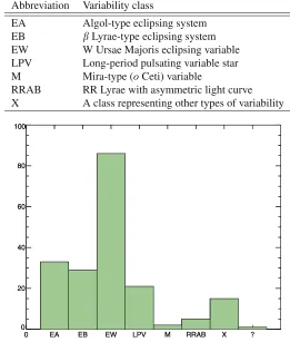
After a careful visual examination of the phase-folded light curves, 192 new periodic variable stars have been detected in the 19hr field of which 185 are previously unknown. Based on the morphology of the light curves, the stars were classified into various variability classes, summarised in Table1. Figure2 presents a histogram of the number of detected variables classified as belonging to each of the types.
The majority of the periodic variable stars detected are eclipsing binaries of various types: all of them make up to more than 75% of the variable stars detected. The following biggest group is the long-period variables. As it can be observed on the histogram presented on the left panel of Fig.3, the majority of detected variable stars have periods ranging from less than a day to about four days. However, the group of long-period variable stars with periods over 100 days can also clearly be identified on the right-hand end of the histogram. The values of the median magnitudes of the detected variable stars range from
Table 1. Variability classes used in the Catalogue of periodic variable stellar sources in the 19hr field of the Wide
Field Transit Survey.
Abbreviation Variability class
EA Algol-type eclipsing system EB Lyrae-type eclipsing system EW W Ursae Majoris eclipsing variable LPV Long-period pulsating variable star M Mira-type (oCeti) variable
RRAB RR Lyrae with asymmetric light curve X A class representing other types of variability
EA EB EW LPV M RRAB X ?
0 0 20 40 60 80 100
EA EB EW LPV M RRAB X ?
0 0 20 40 60 80 100
Figure 2. A histogram of the number of stars classified as belonging to the different variability classes. See text for
details on type X.
−1 0 1 2 3
Log Period 0 20 40 60 80
11.8 12.8 13.9 15.0 16.0 17.1 18.2 19.2 J Magnitude 0 5 10 15 20 25 30
Figure 3. Left panel: histogram of the logarithm of the periods of the detected variable stars; Right panel: histogram
Figure 4. Left panel: logarithm of the amplitude of the first harmonic versus the logarithm of the frequency;
Right panel: two-dimensional projection of the frequency and the phase difference parameter space. The x-axis
represents the frequency in cycles per day and the y-axis – the phase difference between the first two harmonics of the frequency.
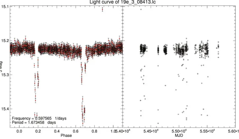
Figure 5. A detached contact binary found in the database with clearly defined primary and secondary minima.
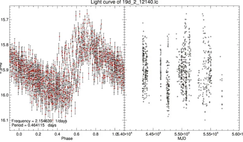
Figure 6. One of the asymmetric periodic variables of type RR Lyr discovered in the database.
definition of the set of parameters of those specific classes so that the new objects in the database are assigned to one of them with a certain probability. For this, let us explore the behaviour of some of the parameters presented, in particular, the frequency, the amplitude, the phase differences between the first two harmonics of the frequency (21=arctan(sin(arctan2−arctan1), cos(arctan2−arctan1))+
/2) and the ratio between the amplitudes of the first two harmonics (R21=A2/A1), in various parameter spaces.
On the left panel of Fig.4 the logarithm of the amplitude of the first harmonic is plotted against the logarithm of the frequency. Based on this, one can clearly separate the long-period variables from the remaining of the classes, but it is difficult to determine any clustering of other classes of variable objects. On the right panel of Fig. 4the frequency is plotted versus the phase difference between the first two harmonics of the frequency (21). What we can observe is that whereas for low frequencies it is not trivial for any clear relation to be detected, the high-frequency domain is dominated by eclipsing binaries of all three classes with21≈0. This is in accordance with the results from the analysis of the Hipparcos archive presented in [10].
Due to ambiguity in the determination of class allocation based merely on the morphology of the light curves, the variability class X contains objects which may belong to various types, among which are cepheids, ellipsoidal variables and spotted stars showing rotational variability. A study of the spectral energy distributions (SED) of the objects has been initiated and the primary results lead to the conclusion that even though some candidates may present features which could be interpreted as belonging to other variability classes, such asScu,Dor, or SPB, they can be rejected due to the results of the SED fitting performed.
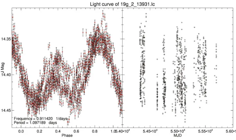
Figure 7. A variable star with a period of 1.09 days that we were unable to classify.
5. CONCLUSIONS
We have presented the detection and morphological classification of 185 new variable stars in the WFCAM Transit Survey based on near-IR photometry. Moreover, we also confirm the the classification and periods of another seven stars that are already in the VSX catalogue [11].
The results can be used as a base for creating a training set for the supervised classification of the rest of the WTS fields so that at the end, the periodic variable stars detected in the survey may present a full set for variable star classification in the near-IR.
HS is supported by RoPACS, a Marie Curie ITN funded by the Seventh Framework Programme of the European Commission. This research has been funded by Spanish grants AYA2012-38897-C02-01, and PRICIT-S2009/ ESP-1496.
References
[1] L. Eyer, J. Cuypers, Predictions on the Number of Variable Stars for the GAIA Space Mission
and for Surveys such as the Ground-Based International Liquid Mirror Telescope, in IAU Colloq. 176: The Impact of Large-Scale Surveys on Pulsating Star Research, edited by L. Szabados, D.
Kurtz (2000), Vol. 203 of Astronomical Society of the Pacific Conference Series, pp. 71–72 [2] J. Birkby, B. Nefs, S. Hodgkin, G. Kovács, B. Sip˝ocz, D. Pinfield, I. Snellen, D. Mislis, F. Murgas,
N. Lodieu et al., MNRAS 426, 1507 (2012) [3] M. Irwin, J. Lewis, New Astronomy 45, 105 (2001)
[5] S.T. Hodgkin, M.J. Irwin, P.C. Hewett, S.J. Warren, MNRAS 394, 675 (2009) [6] P. Vaníˇcek, ApSS 12, 10 (1971)
[7] J.D. Scargle, ApJ 263, 835 (1982)
[8] F.M. Zerbi, R. Garrido, E. Rodriguez, K. Krisciunas, R.A. Crowe, M. Roberts, E.F. Guinan, G.P. McCook, J. Sperauskas, R.F. Griffin et al., MNRAS 290, 401 (1997)
[9] J. Debosscher, L.M. Sarro, C. Aerts, J. Cuypers, B. Vandenbussche, R. Garrido, E. Solano, A&A 475, 1159 (2007)
[10] L.M. Sarro, J. Debosscher, C. Aerts, M. López, A&A 506, 535 (2009)