A MATHEMATICAL MODELLING OF TRANSIENT CURRENT IN AN ELECTRICAL OSCILLATORY SYSTEM

GSJ: Volume 6, Issue 1, January 2018, Online: ISSN 2320-9186

www.globalscientificjournal.com

A

MATHEMATICAL

MODELLING

OF

TRANSIENT

CURRENT

IN

AN

ELECTRICAL

OSCILLATORY

SYSTEM

ATOKOLO, W.

DEPARTMENT OF MATHEMATICAL SCIENCE, KOGI STATE UNIVERSITY, ANYIGBA. E-MAIL:[email protected] PHONE: 08058484474, 07066784329.

ABSTRACT

Mathematical modelling of transient current in an Electrical Oscillatory System, a case of Resistive, Inductive and a Capacitive (RLC) circuit is presented in this research work. The governing equation was formulated from the RLC circuit with the use of Kirchoffs Voltage law (KVL) which is a second order differential equation. The model was then solved taken into consideration four (4) different conditions of the RLC circuit, which includes: the damped, Under-damped, Over-damped and critically damped. Result shows that the circuit is

Un-damped if

R



0

, it is Under-damped (non-oscillatory) if

2

C

L

R



, it is Over-damped (oscillatory) if

2

C

L

R



and it becomes critically damped when

2

C

L

R



respectively.

DEFINITIONS OF VARIABLE USED



i

_{ t} = Transient Current



V

= Voltage or electromotive force in volts



R

= Resistance in ohms (Ω)



L

= Inductance in Henry (H)



= Change in current with time



V

_L = Voltage across the inductor



V

_R = Voltage across resistance



V

_C = Voltage across capacitor

 Root



RLC

= Resistive, Inductive and a Capacitive circuit





_{= Alpha}  e = Exponential





=Gamma



k

k

,

A

2

,

1

and

B

are constants



L

_R=Resistance in an inductive circuit

A simple electric circuit is a closed connection of batteries and wires (Eugene 1996). Transient is the response which occurs in a system leading to change or impulse and then finally dies down after a passage of time (John 2010). The rising and falling of current in a circuit is called Growth and Decay of electric circuit respectively.Atokolo & Omale (2014).

An RLC circuit is an electrical circuit consisting of a resistor (R), an Inductor (L) and a Capacitor (C), connected in a series or in parallel. This type of circuit is an example an Electrical Oscillatory System that practically forms a Harmonic Oscillator for current and resonates in a similar way as an LC circuit. The introduction of the Resistor(R), makes the induced oscillations in the circuit to die away over time if it is not kept going by a source. Anuj (2013), that is to say, the increase in the decay of oscillations caused by the introduction of the Resistor(R), is called Damping.

Theraja (2005)describes Transient as the response which occurs in a system leading to change or impulse and then finally decays after a passage of time. The responses of network containing only resistances and sources have been shown by the Authors to be constant and time invariant. The response of network containing capacitance and inductance is time varying because of the necessary exchange of energy between capacitor and inductive elements. RLC circuit, which is an example of an Electrical Oscillatory system, utilizes double energy transient, the electromagnetic and the electrostatic, any sudden change in the circuit involves in the redistribution of the two forms of energy, the transient current produced due to this redistribution is called double energy transient.Theraja (2005).

This circuit has many applications, among which are: the selection of a certain narrow range of frequencies from the total spectrum of ambient radio waves, for instance, AM/FM Radios with analogue tuners typically use an RLC circuit to tune a radio frequency, most commonly, a variable capacitor is attached to the tuning knob which allows one to change the value of capacitance in the circuit and tune to stations on different frequencies. Milford (1995). The RLC circuit in this case acts as a tuned circuit mostly used today in broadcasting stations. The RLC circuit can also be used as a filter, the RLC filter is described as a second order circuit meaning that any voltage or current in the circuit can be described by a second order differential equation in circuit analysis. Frank (2008).

Resonate frequency is defined as the frequency at which the impedance is purely resistive, this occurs because the impedances of the inductor and capacitor are equal but of opposite sign and as such cancels out. Frank (2008).

2.0 FORMULATION OF PROBLEM

The RLC circuit posses double energy transient; there are the electromagnetic and electrostatic. Any sudden change in the circuit involves in the redistribution of the two forms of energy. The transient currents produced due to this redistribution are known as double energy transient. The transient current can be a unidirectional form or inform of decaying oscillatory current.

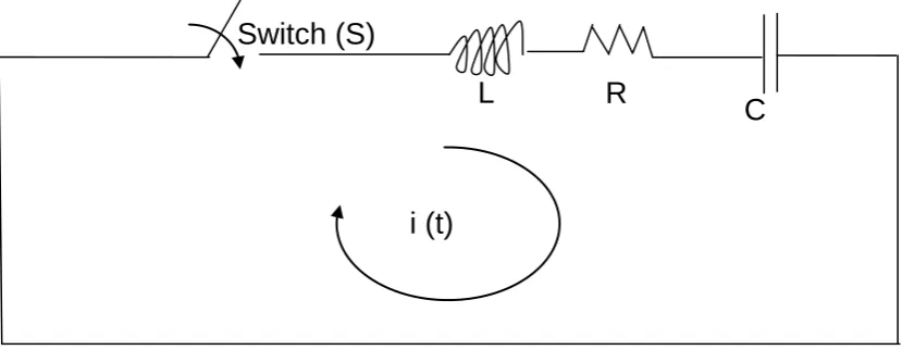
Consider an R.L.C. circuit having a resistance R (



), Inductance L(H) and capacitance C(f) as shown in the diagram below:

FIG 1: RLC CIRCUIT

If there is a sudden change in the circuit that is, if switch S is closed, the redistribution of voltage and current is given by the equation below which is got by the use of kirchoffs voltage law (KVL):

0







C

V

L

V

R

V









1

idt

0

C

dt

di

L

Ri

--- (2.0)

Differentiating equation (2) gives

0

2

2







c

i

dt

Rdi

dt

i

d

L

……….(2.1)

Dividing all by L gives

0

2

2







Lc

i

Ldt

Rdi

dt

i

d

--- (2.2)

This is a second order differential equation which is the formulated problem that requires solutions.

3.0 SOLUTION TO THE PROBLEM

From equation (2.1) above, forming an auxiliary equation or characteristics equation for the above second order differential equation gives

0

1

2

_

_

_

LC

m

L

R

m

,

That is to say

2

2

2

m

dt

i

d

_

,

m

dt

di

_

and

i



1

L

R

C

Switch (S)

0

1

2

_

_

_

LC

m

L

R

m

--- (3.0)

LC

m

L

R

m

2







1

This is a quadratic equation, now solving this equation using completing the square method gives:

2

4

2

1

2

4

2

2

L

R

LC

L

R

m

L

R

m











LC

L

R

L

R

m

1

2

4

2

2

4

2

2

_

_

_





_











2

2

L

R

m

LC

L

R

1

2

4

2



Taking square root of both sides yield





























_

_

_

_

LC

L

R

L

R

m

1

2

4

2

2

2

or ---(3.1)





























_

_

_

_

LC

L

R

L

R

m

1

2

4

2

2

2





























_

_

_

_

LC

L

R

L

R

m

1

2

4

2

2

Or--- (3.2)





























_

_

_

_

LC

L

R

L

R

m

1

2

4

2

2

Therefore:

























LC

L

R

L

R

m

1

2

4

2

2

























LC

L

R

L

R

m

1

2

4

2

2

2

The term under the square root is called the discriminant. The value of the discriminant determines the condition of the circuit, depending on the value of

m

₁ and

2

m

.

Four different conditions of the circuit are distinguishable which are examined as follows in the case of RLC circuit.

CASE 1: UN-DAMPED CONDITION (NO LOSS FREE CIRCUIT, R=0)

In this case, R=0, then equation (3.3) becomes:

LC

m

₁







1

And

LC

m

1

2







Therefore,

LC

j

m

₁



1

And

LC

j

m

1

2





Let

LC

w



1

That is to say:

jw

m

₁



And

m

₂





jw

Recalling the solution of the above second order equation

0

2

2







c

dx

dy

b

dx

y

d

a

The solution of the above second order ODE is given by

x

m

B

x

m

A

y





1





2 _{--- (3.4)}

Where A and B are arbitrary constants which depend on some boundary conditions. Applying this to our formulated problem in equation (2.0) we have

t

m

k

t

m

k

t

i

2

2 1 1

)

(









--- (3.5)

Since

m

₁



jw

and

m

2





jw

jwt

k

jwt

k

t

i











2 1

)

sin

cos

)

sin

(cos

(

)

(

t

k

₁

wt

j

wt

k

₂

wt

j

wt

i









wt

k

k

j

wt

k

k

t

i

(

)

(

)

cos

(

)

sin

2 1 2

1









Where

2

1

k

k



= A and

(

)

2

1

k

k

j



= B

Therefore

i

(

t

)



A

(cos

wt



B

sin

wt

)

--- (3.6)

Equation (3.6) is the solution for the un-damped circuit condition

CASE 2: UNDER-DAMPED CONDITION (LOW LOSS CIRCUIT)

In this case,

LC

L

R

1

2

4

2



, the circuit does not oscillates, in other words, the period of oscillations decreases,

1

m

and

2

m

form a complex roots. Dass & Rama (2008).

























LC

L

R

L

R

m

1

2

4

2

2

1 --- (3.7)

























2

4

2

1

2

1

L

R

LC

L

R

m

j

Or

























2

4

2

1

2

2

L

R

LC

L

R

m

j

This is because

LC

L

R

1

2

4

2



Let

L

R

2



=



and



















2

4

2

1

L

R

LC

=

w

1

m

=



+

jw

and

2

m

=



-

jw

Now substituting the values into the general equation (3.5)

t

m

k

t

m

k

t

i

2 2 1 1

)

t

jw

k

t

jw

k

t

i

(

)

(

)

(

)

2 1

















jwt

t

k

jwt

t

k

t

i





















2 1

)

(

]

[

2 1

)

(

t

t

jwt

jwt

i







k





k





But



jwt



cos

wt



j

sin

wt

)]

sin

(cos

)

sin

(cos

[

)

(

2

1

wt

j

wt

k

wt

j

wt

k

t

t

i













]

sin

)

(

cos

)

[(

)

(

t

t

k

₁

k

₂

wt

j

k

₁

k

₂

wt

i













Where

2

1

k

k



=A and

(

)

2

1

k

k

j



=B

]

sin

cos

[(

)

(

t

t

A

wt

B

wt

i









--- (3.8)

Where





t

= Damping factor and



is taken as

L

R

2

Also if



is taken as

L

R

2



then we have:

]

sin

cos

[(

)

(

t

t

A

wt

B

wt

i











Else:

]

sin

cos

[(

)

(

t

t

A

wt

B

wt

i









--- (3.9)

Equation (3.9) is the solution for the under-damped circuit condition

The term







t

is called the damping factor which accounts for the decay of oscillation. The frequency of the damped oscillation is given by





















2

4

2

1

L

R

LC

F

is called the natural frequency of the circuit.

If

2

4

2

L

R

<<

LC

1

, that is if

2

4

2

L

R

is far far less than

CASE 3: OVER-DAMPED CONDITION (HIGH LOSS CIRCUIT)

In this case,

2

4

2

L

R

is >

LC

1

, the circuit oscillates, in other words, the period of oscillations increases.

m

₁

And

m

2 will be unequal. Dass & Rama (2008) From equation (4):

























LC

L

R

L

R

m

1

2

4

2

2

1 Or

























LC

L

R

L

R

m

1

2

4

2

2

2

L

R

2

=



and



















LC

L

R

1

2

4

2

=



1

m

=





+



and

2

m

=









--- (3.91)

To find the solution of the differential equation, we substitute (3.91) into the general equation (3.5) we have:

t

k

t

k

t

i

(

)

(

)

(

)

2 1











_









_

_

t

t

k

t

t

k

t

i



























2 1

)

(

]

[

2 1

)

(

t

t

t

t

i









k







k







Converting this to a hyperbolic function, that is





t



cosh



t



sinh



t

)]

sinh

(cosh

)

sinh

(cosh

[

)

(

2

1

t

t

k

t

t

k

t

t

i























]

sin

)

(

cos

)

[(

)

(

t

t

k

₁

k

₂

wt

j

k

₁

k

₂

wt

i















Where

2

1

k

k



=A and

(

)

2

1

k

k

]

sinh

cosh

[(

)

(

t

t

A

t

B

t

i















--- (3.92)

CASE 4: CRITICALLY-DAMPED CONDITION

It is a special case of damping, which is the minimum damping that can be applied to a circuit or a system without causing oscillations.

In this case,

2

4

2

L

R

=

LC

1

, That is to say,



2

4

2

L

R

0

1

_

LC

From equation (3.3),

L

R

m

m

2

2

1







putting this value into the general equation (3.5) which is given by

t

m

k

t

m

k

t

i

2

2 1 1

)

(









gives

L

Rt

L

Rt

K

k

t

i

2

2

2

1

)

(













Where

L

R

2





]

[

)

(

t

t

k

₁

k

₂

i











--- (3.93)

Therefore, the solutions of the formulated problem under the four (4) conditions are simply represented by equations (3.6), (3.9), (3.92) and (3.93) respectively, these are

)

sin

(cos

)

(

t

A

wt

B

wt

i





--- --- (3.6)

]

sin

cos

[(

)

(

t

t

A

wt

B

wt

i









--- (3.9)

]

sinh

cosh

[(

)

(

t

t

A

t

B

t

i















--- (3.92)

]

[

)

(

2

1

k

k

t

t

i











--- (3.93)

4.0 ANALYSIS OF THE MODEL

20

10

05

.

0

718

.

2

5

.

0

05

.

0

20

10

2 1



















k

k

r

e

Z

w

B

A



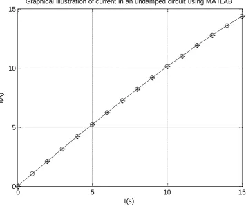
The graphical illustrations for current in un-damped, under-damped, over-damped, critically damped circuits are given below using Mat-lab.

Figure 2:Graphical illustration of current in an undamped circuit

0 5 10 15

0 5 10 15

t(s)

i(

A

)

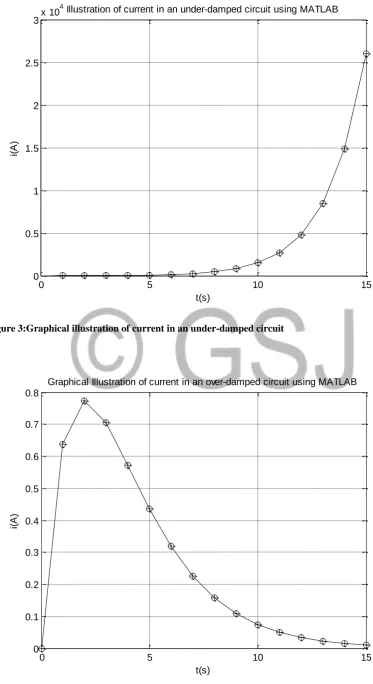
Figure 3:Graphical illustration of current in an under-damped circuit

0 5 10 15

0 0.5 1 1.5 2 2.5

3x 10

4

t(s)

i(

A

)

Illustration of current in an under-damped circuit using MATLAB

0 5 10 15

0 0.1 0.2 0.3 0.4 0.5 0.6 0.7 0.8

t(s)

i(

A

)

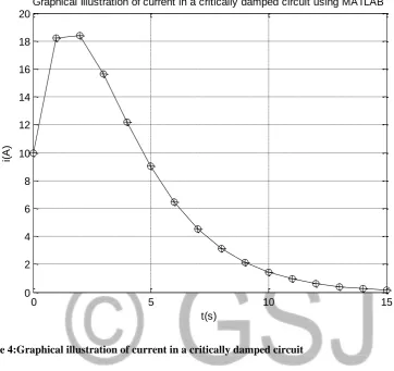
Figure 4:Graphical illustration of current in a critically damped circuit

From the un-damped graphical illustration above, a plot of current (i) against time (t) shows that the current increases as the time increases linearly. The under- damped graphical illustration shows that the current maintains a steady state value at about 0-7 seconds, a little increment in the current (i) brings about an increase in the time(t). Over- damped and the critically damped graphical illustrations show that the current has no steady state value as the current (i) decreases with an increase in time (t).

5.0 CONCLUSION

Mathematical modelling of transient current in an Electrical Oscillatory System, a case of Resistive, Inductive and a Capacitive (RLC) circuit is presented in this research work. Result shows that the circuit is Un-damped if

0



R

, it is Under-damped (non-oscillatory) if

2

C

L

R



, it is Over-damped (oscillatory) if

2

C

L

R



and

it becomes critically damped when

2

C

L

R



respectively.

0 5 10 15

0 2 4 6 8 10 12 14 16 18 20

t(s)

i(

A

)

REFERENCES

Anuj, S. (2013). Transient Analysis of Electrical Circuits using Runge Kutta method and its application. School of Mechanical and Building Sciences VIT, University. ISSN, Volume 3, issue 11, Pp2-5.

Atokolo, W. & Omale, D.(2015).Mathematical modelling of Growth and Decay of Electric current.Department of Mathematical Sciences, Kogi State University Anyigba.Pp.2-7

Dass,H.K. & Rama, V.(2008). Mathematical Physics,

S. Chand & Company PVT.LTD. Ram Nagar, New Delhi-110055.Pp424-428. Eugene H. (1996) Physics Calculus, Brooks/Cole Publisher 2nd edition. Pp754. Frank, Y.W. (2008) Physics with Maple: the computer Algebra

John B. (2010). Electric Circuit theory & Technology, 4th edition, Newness publishers Pp. 9, 155, 229.

Milford, F.J. Reitz, J.R. Christy, R.W.(1995), fundamental of Electromagnetic theory, New York: Addison-Wesley.

Thereja B.L (2005), A textbook of electrical technology.

Sixth edition 2001, page 189 – 231. S. Chand and company Publisher

APPENDIX: MATLAB CODES CODES FOR CURRENT IN AN UN-DAMPED CIRCUIT

c = B*sin(a); i = a+c; plot(t,i,'k') hold on plot(t,i,'+k')

hold on; plot(t,i,'ok') xlabel('t(s)')

ylabel('i(A)')

title('Graphical Illustration of current in an undamped circuit using MATLAB') grid on

CODES FOR CURRENT IN AN UNDER-DAMPED CIRCUIT

t = [0:15]; A = 10; B = 20; Z=0.5; e=2.718; m =(t*Z); q = e.^m; W = 0.05; a = W*t; b = A*cos(a); c = B*sin(a); f = a+c; i= q.*f; plot(t,i,'k') hold on plot(t,i,'+k')

hold on; plot(t,i,'ok') xlabel('t(s)')

ylabel('i(A)')

title('Illustration of current in an under-damped circuit using MATLAB') grid on

CODES FOR CURRENT IN AN OVER-DAMPED CIRCUIT

t = [0:15]; A = 10; B = 20; Z=0.5; e=2.718; m=-(t*Z); q = e.^m; r = 0.05; a = r*t; b = A*cosh(a); c = B*sinh(a); f = a+c; i= q.*f; plot(t,i,'k') hold on plot(t,i,'+k')

hold on; plot(t,i,'ok') xlabel('t(s)')

ylabel('i(A)')

CODES FOR CURRENT IN A CRITICALLY-DAMPED CIRCUIT

t = [0:15]; K1 = 10; K2 = 20; e = 2.718; z=0.5 a = -(t*z); p = e.^a; s = K2*t; q = (K1+s) i = q.*p; plot(t,i,'k') hold on plot(t,i,'+k')

hold on; plot(t,i,'ok') xlabel('t(s)')

ylabel('i(A)')