Application of Sobol’s Method for Parametric Study of a Robotic Manipulator with Two Flexible Links

©2013 JNAS Journal-2013-2-10/489-497 ISSN 2322-5149 ©2013 JNAS

Application of Sobol’s Method for Parametric

Study of a Robotic Manipulator with Two Flexible

Links

M. H. Korayem

1*

, A. M. Shafei

2

and A. Azimi

3

1- Professor of Mechanical Engineering Department, Iran University of Science and Technology, Narmak, Tehran, Iran

2- Ph.D. Candidate of Mechanical Engineering Department, Iran University of Science and Technology, Tehran, Iran

3- M.Sc. Student of Mechanical Engineering Department, Iran University of Science and Technology, Tehran, Iran

Corresponding author: M. H. Korayem

ABSTRACT: The paper’s focus is on studying the sensitivity analysis (SA) of the geometric parameters

(including length, thickness and width) of a robotic manipulator with two elastic links. Two important parameters that influence the design of these kinds of robotic systems are the maximum deflection (MD) of the end-effector and the vibration energy (VE) of that point. So, the Sobol’s SA method is applied to determine how these two parameters are influenced by the geometric parameters of the system. The dynamic model of the system is developed based on the Lagrangian formulation. Elastic properties of the links are modeled by applying the Assumed Modes Method (AMM) and the assumption of the Euler Bernoulli Beam Theory (EBBT). Finally, based on the achieved results, a parameter is introduced as a criterion to design the elastic robotic manipulators with the least adverse effects of vibration.

Keywords: Maximum Deflection, Vibration Energy, Euler-Bernoulli, Sensitivity Analysis, Sobol.

INTRODUCTION

Research into the elastic manipulator fields has become more important for many years on account of the new robotic applications in various fields such as: industrial tasks in which the trend is to use lightweight materials. Nowadays, most of the existing robots are built by using the heavy materials and bulky design to minimize the vibration of the end-effector to achieve the acceptable accuracy. The rigid manipulators are not efficient in terms of power consumption or speed. As a consequence, building the robotic manipulators in a lightweight design is very desirable to reduce the weight of the arms to increase their speed of operation. So, understanding and analyzing of flexible manipulations has concerned researchers for many years (Nikolakopoulos et al., 2010; Hassan et al., 2007; Bascetta et al., 2006; Korayem et al. 2005; Hermle et al., 2000).

SA is an essential instrument for designing, building, use and understanding of mathematical models of all forms (Taranatola et al., 2003). Investigators have accepted that the SA of complicated phenomena are very important and essential to overall analysis of such phenomena (Turanyi, 1990). The main goal of the SA is to identify the most significant factors among the others that contribute in the output variables (Storlie et al., 2009; Kucherenco et al., 2008; Xu et al., 2007). Parametric study has been used widely in other sciences to analyze models (Ellwein et al., 2008; Richter et al., 2009; Korayem et al., 2009; Korayem et al., 2010), but this type of analysis has been used the least for the analysis of the elastic robotic manipulators.

490

effects of all geometrical parameters on vibrations and deflections of the end-effector (Korayem et al., 2012). But as mentioned, this study was confined to single flexible link. In this manuscript to design the optimal dimensions for a two links elastic robotic manipulator, the parametric study of this system will be investigated by Sobol’s SA method. So, the rest of the paper is gorgonized as following:

At first, motion equations of a two links flexible manipulator will be derived according to the Lagrangian formulation and AMM. Then VE and MD of the end-effector are obtained using EBBT theory. In continue Sobol’s SA method is used to evaluate how VE and end-point MD are influenced by geometric parameters. Finally, the conclusions from the present work are summarized and the merits of the proposed method are highlighted.

Modeling of a Manipulator with Multiple Flexible Links

The generalized Euler-Lagrange formulation and assumed modes method is used to derive the dynamic equations of flexible manipulators. All the flexible links are assumed to be Euler-Bernoulli beams, where the shear-force-shortening effect and rotary inertia are neglected. For a general N-link flexible robot, the vibration vi xi,t of

each link which describes the deflection of the ith link with respect to its undeflected configuration can be represented by a series form as

 



_

ni_

   



j ij i ij

i

i x t x q t i n

v

1 , 1,...,

,  (1)

Where vi

 

xi,t _{is the bending deflection of the i}th _{link at a spatial point} xi



0xiLi,t



_and Li _{is the length of the i}th

link.

n

i _{is the number of modes used to describe the deflection of link i;} ij

 

xi _and qij

 

t _{are the j}th _{mode shape}

function and jth modal displacement for the ith link, respectively. Position and velocity of each point on link I can be

obtained with respect to inertial coordinate frame using the transformation matrices between the rigid and flexible coordinate systems. After that, by considering the generalized coordinates of the manipulator which consists of two

parts, the generalized coordinates of the rigid body motion of the links





T n r q q q q  ₁, ₂,...

and generalized coordinates

defining the deflection of the manipulator





T nn n n n

f q q q q q q q n

q ₁₁, ₁₂,..., ₁, ₂₁,..., ₂ ,..., ₁,...,

2 

, the dynamic equation of flexible link manipulator is developed by using the Lagrangian assumed modes method as follows:

















. , , ,

, ,

, , ,

   

      

            

 

f r f

f r r

f r f r f

f r f r r

f r

ff fr

rf rr

q q H

q q G q q q q H

q q q q H q q m m

m m

 

  

  

(2)

By defining the generalized forces as

  



T n

i U

U  1,2,..., ,0,...,0 _{and, the generalized coordinate system as}

 





T

nn n

n n n

i q q q q q q q q q n

Q

Q ₁, ₂,..., , ₁₁,, ₁₂,..., ₁ ,..., ₁, ₂,...,

1

 

, where i1,...,ntnn1n2...nn_{, Eq.(2) can be}

written in compact form as

 

Q,Q G

 

Q U,

H Q

M    (3)

where M is the mass matrix, H is the vector of Coriolis and centrifugal forces, and G describes the gravity effects. By defining the following vectors as

 

 

 

 

 

,

 

; 1,...,2 , ,...,

1 ;

, ,

,

2 2

1 2 1 2

2 1

2 1

t i

i

t i

i i

i

n i

f F x X

n i

f F

f F Q x X Q x X

  

 

   

   

(4)

Eq.(3) can be expressed in terms of the following state equation

 



,



,

; 2 2 1 1 2

2 1

1 F X X F D X U N X X

X       (5)

where DM1 _and





1 2



 

1



1

,X G X

X H M

N   _.

Deriving the motion equations

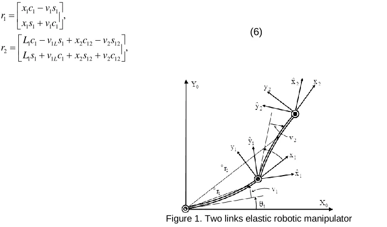
A two-link manipulator with flexible link at horizontal plane with the associated coordinate system is shown in Figure1. Using the generalized modeling scheme, equations of motion of a manipulator with two flexible links are derived here.

Using the symbols defined in Figure1, the expressions for position vector r1 and r2 in the XY plane can be written

491 , , 12 2 12 2 1 1 1 1 12 2 12 2 1 1 1 1 2 1 1 1 1 1 1 1 1 1                       c v s x c v s L s v c x s v c L r c v s x s v c x r L L (6)

Figure 1. Two links elastic robotic manipulator

where c1,s1,c12 and s12 are shorthand expressions for cos

   

1,sin1,cos



12



, and sin



12



, respectively. To

obtain a simplified model with reasonable accuracy, two modes per link are considered, so vi

 

xi,t _{can be given by}

   

   

   

   

   

   

   

   

, , , , 22 2 22 21 1 21 2 12 1 12 11 1 11 1 22 2 22 21 1 21 2 12 1 12 11 1 11 1 t q L t q L v t q L t q L v t q x t q x v t q x t q x v L L                 (7)

By considering the simply support mode shape,



ij _{can be computed as follows:}

 

xi sin



j xi/Li



, i1,2andj1,2.

ij 

 (8)

The kinetic energy of a point ri

 

xi _{on the links can be written as}

   

   

, 5 . 0 , 5 . 0 2 2 2 0 2 2 2 2

1 1 1 0 1 1 1 1 2 1 dx x r x r K dx x r x r K L T L _T    





    (9)

Where



i _{is the linear mass density for the i}th

link and

r



i

 

x

i _{is the velocity vector. The velocity vector can be}

computed by taking the time derivative of its position (6):

















, , 12 2 1 2 12 2 12 2 1 2 1 1 1 1 1 1 1 1 12 2 1 2 12 2 12 2 1 2 1 1 1 1 1 1 1 1 2 0 1 1 1 1 1 1 1 1 1 1 1 1 1 1 1 1 1 0                                  s v c v c x c v s v c L c v s v s x s v c v s L r c v s v c x s v c v s x r L L L L                                         (10)

On the other hand, the potential energy due to the deformation of the first and second links can be written as





      2 1

0 2 2

2 2 2 2 2 2

0 2 1

1 1 2 1 1 1 , 2 1 , 2 1 L L dx x v I E U dx x v I E U (11)

where

E

i

I

i _{is the flexural rigidity of the i}th _{link and}

v

i _{is substituted from (7) and (8). Next, to obtain a closed-form}

dynamic model of the manipulator, the energy expressions (9) and (11) are used to formulate the Lagrangian



1 2



2

1

K

U

U

K

492

displacements



q11,q12,q21,q22



_{. The generalized force vector is}





T

U 1,2,0,0,0,0 _{, where}



1 _and



2 _{are the torques}

applied by motor 1 and motor 2, respectively. Therefore, the following Euler-Lagrange’s equations results, with 2

, 1 

i _and j1,2_:

. 0 , 0 , 2 2 1 1                                         j j j j i i i q L q L dt d q L q L dt d L L dt d    _   (12)

The final dynamic equations of motion of the manipulator after algebraic simplifications can be put in a concise form as , 0 0 0 0 2 1 22 21 12 11 2 1 22 21 12 11 2 1 44 34 33 24 23 22 14 13 12 11 214 213 212 211 22 114 113 112 111 12 11                                                                                  









f f f f r r ff ff ff ff ff ff ff ff ff ff rf rf rf rf r rf rf rf rf r r h h h h h h q q q q J J J Sym J J J J J J J J J J J J J J J J J J             (13)

Because of the very long terms of the Coriolis and centrifugal forces, they are neglected to bring in the paper

text. Since the motion is in horizontal plane, the gravity effects



Gr,Gf



_{will be zero. By using Eqs. (3)-(5) and}

defining the state vector as







2 4 6 8 10 12



,

2 11 9 7 5 3 1 1 T T T T x x x x x x Q X x x x x x x Q X      (14)

The state-space form of Eq. (13) is written as

 

; 1,...,6, , 2 2

2 1

2 x x F i i

x i i  i (15)

where F2

 

i can be obtained from eq. (5). Now, by having the governing equations of this robotic system the

parametric study of this system will be studied.

Sobol’s Sensitivity Analysis Method

Sobol’s sensitivity analysis method is used successfully to non-linear mathematical models as a kind of the well-known statistical methods. (Gloda et al., 2008) showed that, Sobol’s method can be applied for model based analysis of robotic systems, efficiently. The input factors region should be determined as follows to explain the Sobol’s method. ,...,k) , ;i x X (

Ωk _i

2 1 1

0  

 (16)

where

x

i _{is the vector of input factors. These vectors are perpendicular with respect to each other. Based on the}

Sobol’s method, the function f(x) _{will be obtained by adding the following functions;}

) ,...,x ,x (x f ... ) ,x (x f ) (x f f ) ,...,x ,x

f(x _{, ,...,k k}

k j

i ij i j

k

i i i

k 0 1 1 12 1 2

2

1  



 



    (17)

In above equation the first term can be determined as,





k

Ω

f(x)dx

f0 ₍₁₈₎

Sobol demonstrated that, the decomposition of Equation (17) is unique. So, all the terms of this equation can be evaluated via multidimensional integrals,





   1 0 1 0

0 ... f(x)dx

f ) (x

fi i (19)





 

   1 0 1 0

0 i i ~ij

j i

ij(x,x ) f f(x) ... f(x)dx

f (20)

where dx~i,dx~ij _{show the integration over all the variables excluding} xi _and xj _{respectively. Consequently, for}

higher-order terms, continuous formula will be attained. In sensitivity indices, the total variance of f(x) _{“ D”, can be}

493

Squaring and integrating of Equation (17) over all variables, may lead to the simplification of expression

D

as:





 

 

 k

i i j k

,...,k , ij

i D D

D D

1 1

2

1 (22)

So the sensitivity magnitudes

S

1,2,...,k_{, are given by:}

D D S ,....,k

,...,k ,

2 1 2

1  1i1...isk (23)

The summation of all the sensitivity indices involving the factor in Equation (23) may lead to the total SA index. By applying the Sobol’s SA the optimal value of the dimensions of the flexible links in order to minimize the vibration energy (VE) and end-effector’s maximum deflection (MD) will be obtained.

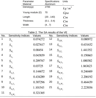
Sensitivity Analysis of the VE

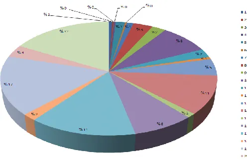
In this section, the assumption of EBBT is used to obtain the VE of the end-effector for both flexible links of the manipulator. At first, the variation intervals of each parameter should be extracted. Table 1, presents those intervals. Then, Sobol’s sampling method is applied to generate 1040 uniform random numbers on the presented intervals in Table1. After generating random numbers, the VE of the end-effector is achieved for each extracted number. The results of the SA of the both elastic links of the manipulator are shown in Table 2. Also, the Pie chart diagram associated with the results of the SA of the VE is illustrated in Figures 2.

Table 1. Properties of the links

Parameter Specifications Units

Material Aluminum -

Density(ρ) 2700 3

/m kg

Young module (E) 70 _Gpa

Length (20 , 140) _Cm

Thickness (0.1 , 0.4) _Cm

Width (4 , 7) _Cm

Table 2. The SA results of the VE

No. Sensitivity Indices Values No. Sensitivity Indices Values

1 1 L

S 0.074272 12

1 1W T

S 0.080972

2 1 T

S 0.027617 13

2 1L T

S 0.631632

3 1 W

S 0.00454 14

2 1T T

S 1.441352

4 2 L

S 0.043839 15

2 1W T

S 0.150663

5 2 T

S 0.209767 16

2 1L W

S 1.080382

6 2 W

S 0.03725 17

2 1T W

S 1.863623

7

1 1T L

S 0.144672 18

2 1W W

S 0.246469

8

1 1W L

S 0.434289 19

2 2T L

S 2.206192

9

2 1L L

S 0.307296 20

2 2W L

S 0.464439

10 2 1T L

S 1.101543 21

2 2W T

S 2.223036

11

2 1W L

494

0.35 0.4 0.45 0.5 0.55 0.6 0.65 0.7

0.005 0.01 0.015 0.02

Length of first link (m)

VE

3 3.2 3.4 3.6 3.8 4

x 10-3 0

0.1 0.2 0.3 0.4

Thickness of first link (m)

VE

0.03 0.035 0.04 0.045 0.05 0.055

-0.05 -0.04 -0.03 -0.02 -0.01 0 0.01 0.02

Width of first link (m)

VE

0.35 0.4 0.45 0.5 0.55 0.6 0.65 0.7 -0.01

0 0.01 0.02 0.03 0.04 0.05

Length of second link (m)

VE

Figure 2. Pie chart diagram of the SA of the VE

According to the Table 2 and Figure 2, it is obvious that among the first sensitive indices, the most percentage of the sensitivity belongs to the thickness of the second link, which is shown by ST2.

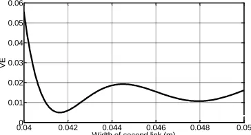
To study the relation of VE and the dimensions of the flexible links, the results are illustrated in Figures 3-8. As it is expected, the results presented in Figures 3-8, show that, to decrease the VE, the elastic link with short length and high width and thickness for each link should be used, except the length of second link. Figure 6 present the changing trend of VE with respect to the second link’s length. As it is shown in figure 6, increasing the length of this link leads to the reduction of the VE. It happens because of the effect of the second link’s thickness on VE. According to the Table 2 and Figure 2, for the second link the effect of thickness is five times more than the effect of the length. Due to the great effect of the second link’s thickness, it is not allowed to the VE to increase with respect to the length. To achieve the best decision of choosing the optimum dimensions due to VE minimization, the factor of L1L2/T1T2W1W2 is defined. Figure 9 shows the relation between VE and L1L2/T1T2W1W2, by using the EBBT

assumption. According to the Figure 9, the best value of L1L2/T1T2W1W2 is about

     

 6 1₂

10 54 . 1

cm _{. Therefore, the}

dimensions of the flexible links should be selected so that the factor of 

    

 2

6 2

1 2 1 2 1

1 10 54 . 1 /

cm W

W T T L L

.

Figure 3. Effect of the first link’s length on VE Figure 4. Effect of the first link’s thickness on VE

495

Figure 7. Effect of the second link’s thickness on VE Figure 8. Effect of the second link’s width on VE

Figure 9. Effect of the L1L2/T1T2W1W2 on VE

Sensitivity analysis of MD of the end-effector

In this section, the MD of the end-effector of the elastic links related to those 1040 extracted random numbers is computed. The SA is done based on Sobol’s method. The corresponding results of SA are presented in Table 3. Figure 10 shows the pie chart diagram of the SA.

Table 3. The SA results of the MD

No. Sensitivity Indices Values (EBBT) No. Sensitivity Indices Values (EBBT) 1

1

L

S 0.04552 12

1 1W

T

S 0.058294

2

1

T

S 0.0557 13

2 1L

T

S 0.0720729

3

1

W

S 0.002635 14

2 1T

T

S 1.58232

4

2

L

S 0.121482 15

2 1W

T

S 0.114416

5

2

T

S 0.387281 16

2 1L

W

S 0.427487

6

2

W

S 0.1483 17

2 1T

W

S 1.177331

7

1 1T

L

S 0.209837 18

2 1W

W

S 0.051412

8

1 1W

L

S 0.058213 19

2 2T

L

S 1.269642

9

2 1L

L

S 0.267382 20

2 2W L

S 0.330195

10

2 1T

L

S 0.896335 21

2 2W

T

S 1.409782

11 SL1W2 0.073477

Figure 10. Pie chart diagram of SA of the MD

1 1.2 1.4 1.6 1.8 2

x 10-3

-0.05 0 0.05 0.1 0.15 0.2 0.25

Thickness of second link (m)

VE

0.040 0.042 0.044 0.046 0.048 0.05

0.01 0.02 0.03 0.04 0.05 0.06

Width of second link (m)

VE

1.55 1.56 1.57 1.58 1.59 x 106 -0.153

-0.152 -0.151 -0.15 -0.149

496

According to the Figure 10, and like the previous Section it is understood that the most effective parameter

among the first sensitivity indices, is ST2, which shows the sensitivity of the second link’s thickness.

To find out how each parameter affects on the MD of the end-effector a simulation is performed. Figures 11- 16 show the results. Each figure shows the relation of MD of the end-effector with respect to the related parameter based on the EBBT assumption.

According to the Figures (11-13), the MD of the end-effector is increased by the growth of the length, but by increasing the amount of thickness and also width, the MD of the end-effector will be reduced. Figures (14-16) show the MD of the end-effector is reduced by increasing all the geometric parameters of the second link. Among these, the behavior of the MD with respect to the second link’s length is not normal. It is because of the effect of the second link’s thickness on MD. As it is noted in Table 3 and shown in Figure 10, for the second link, the effect of thickness is three times bigger than the effect of the length. Because of the high effect of the second link’s thickness, the increasing trend of the MD with respect to the length is observed. So, like the previous Section, to find the optimal values of dimensions to achieve the minimum MD, the factor of L1L2/T1T2W1W2 is defined here. Figure

17 shows the relation between the MD and L1L2/T1T2W1W2. According to the Figure17, the best values of L1L2/T1T2W1W2

is 

    

2

7 1

10 1 . 1

cm _{. As noted, the dimensions of the flexible links should be selected so that} 

    

 2

7 2 1 2 1 2 1

1 10 1 . 1 /

cm W

W T T L L

.

Figure 11. Effects of the first link’s Length on MD Figure 12. Effects of the first link’s thickness on MD

Figure 13. Effects of the first link’s width on MD Figure14. Effects of the second link’s length on MD

Figure 15. Effects of the second link’s thickness on MD Figure16. Effects of the second link’s width on MD

0.45 0.5 0.55 0.6 0.65 0.7

0.15 0.2 0.25

Length of first link (m)

MD

3 3.5 4 4.5 5

x 10-3

0.05 0.1 0.15 0.2

Thickness of firt link (m)

MD

0.03 0.035 0.04 0.045 0.05 0.055

-0.15 -0.1 -0.05 0 0.05 0.1 0.15 0.2

Width of first link (m)

MD

0.350 0.4 0.45 0.5 0.55 0.6 0.65 0.7

0.1 0.2 0.3 0.4 0.5

Length of second link (m)

MD

1 1.2 1.4 1.6 1.8 2

x 10-3

0 0.2 0.4 0.6 0.8 1

Thickness of second link(m)

MD

0.04 0.042 0.044 0.046 0.048 0.05

0.1 0.15 0.2 0.25 0.3 0.35

Width of second link (m)

497

Figure 17. Effects of the L₁L₂/T₁T₂W₁W₂ on MD

CONCULSION

In this research, motion equations of the two flexible links manipulator are extracted by using the Lagrangian formulations. AMM is applied to achieve the elastic modeling of the system. VE and MD of the end-effector are chosen to study their behavior to achieve appropriate criteria for mechanical design of the system. Additionally, all of the simulations are done based on EBBT assumption, and SA is done by using Sobol’s method. After studying the effects of each geometric parameter, the relation between those parameters vs. VE and MD are presented. It is shown that, the most sensitive parameter corresponds to the second link’s thickness. According to the results, the

optimum values of VE and MD occur at 

    

2

6 1

10 54 . 1

cm _and 

    ₁₀7 1₂

1 . 1

cm _for L1L2/T1T2W1W2_{, respectively.}

REFERENCES

Bascetta L, Rocco P. 2006. End-Point Vibration Sensing of Planner Flexible Manipulators through Visual Servoing, 16: 221-232. Ellwein LM, Tran HT, Zapata CH, Novak V, Olufsen, MS. 2008. Sensitivity Analysis and Model Assessment: Mathematical

Models for Arterial Blood Flow and Blood Pressure. Cardiovasc. Eng, 8(2): 94-108.

Gloda D, Lagnema K, Dubowsky S. 2008. Probabilistic Modeling and Analysis of High-Speed Rough Terrain Mobile Robots. IEEE Int. Conf. on Rob. Auto: 914-919.

Hassan M, Dubay R, Li C, Wang R. 2007. Active Vibration Control of a Flexible One-Link Manipulator Using a Multivariable Predictive Controller, 17: 311-323.

Hermle M, Eberhard P. 2000. Control and Parameter Optimization of Flexible Robots. Mechanics of Structures and Machines, 28(2-3): 137-168.

Korayem MH, Basu A. 2005. Dynamic Load Carrying Capacity of Mobile-Base Flexible Joint Manipulators. The International Journal of Advanced Manufacturing Technology, 25(1-2): 62-70.

Korayem MH, Zakeri M. 2009. Sensitivity Analysis of Nanoparticles Pushing Critical Conditions in 2-D Controlled Nanomanipulation Based on AFM. J. adv. Manuf. Tech, 41: 714-726.

Korayem MH, Zakeri M. 2010. The Effect of Off-End tip Distance on the Nanomanipulation Based on Rectangular and V-Shape Cantilevered AFMs. J. Adv. Manuf. Tech, 50: 579-589.

Korayem MH, Shafei AM, Azimi. 2012. Parametric Study of a Single Flexible Link Based on Timoshenko and Euler-Bernoulli Beam Theories. Int. Res. Jour. Appl. Sci, 3: 1535-1543.

Kucherenco S, Fernandez C, Pantelides C. 2008. Monte Carlo Evaluation of Derivative-Based Global Sensitivity Measures. Reliability Engineering and System Safety, 94: 1135-1148.

Nikolakopoulos G, Tzes A. 2010. Application of Adaptive Lattice Filters for Modal Parameter Tracking of a Single Flexible Link Carrying a Shifting Payload. Mechanical Systems and Signal Processing, 24: 1338-1348.

Richter G M, Acutis M, trevisiol P, Latiri K, Confalonieri R. 2009. Sensitivity Analysis for a Complex Crop Model Applied to Durum Wheat in the Mediterranean. Eur, J, Agron, 32: 127-136.

Saltelli A, Chan K, Scott M. 2000. Sensitivity analysis, Wiley Series in Probability and Statistics. New York: Wiley. Sobol IM. 1993. Sensitivity Estimates for Nonlinear Mathematical Models. Math, Model, Comput. Exp, 14: 407-414.

Storlie CB, Swiler LP, Helton JC, Sallaberry CJ. 2009. Implementation and Evaluation of Nonparametric Regression Procedures for Sensitivity Analysis of Computationally Demanding Models. Reliability Engineering and System Safety, 94: 1735-1763.

Taranatola S, Salteli A. 2003. Methodological Advances and Innovative Applications of Sensitivity Analysis. Reliabl. Eng. Syst. Saf, SAMO, 79: 121-122.

Turanyi T. 1990. Sensitivity Analysis of Complex Kinetic Systems. Tools and Applications, Journal of Mathematical chemistry, 5 (3): 203-248.

Xu C, Gertner GZ. 2007. A General First-Order Global Sensitivity Analysis Method. Reliability Engineering and System Safety, 93: 1060-1071.

1.1 1.15 1.2 1.25 1.3 1.35

x 107

0.05 0.1 0.15