Ambient Air Quality Estimation using Supervised
Learning Techniques
Jasleen Kaur Sethi
1, Mamta Mittal
2,*1Research Scholar, University School of Information, Communication & Technology, Guru Gobind Singh Indraprastha University, New Delhi – 110078
2Department of Computer Science & Engineering, G.B. Pant Government Engineering College, New Delhi – 110020
Abstract
The exponential increase of population in the urban areas has led to deforestation and industrialization that
greatly affects the air quality. The polluted air affects the human health. Due to this concern, the prediction of
air quality has become a potential research area. For the assessment of air quality an important indicator is Air
Quality Index (AQI). The objective of this paper is to build prediction models using supervised learning.
Supervised Learning is broadly classified into: classification, regression and ensemble techniques. This study
has been carried out using various techniques of classification, regression and ensemble learning. It has been
observed from experimental work that Decision Trees from classification, Support Vector Regression from
regression and Stacking Ensemble from ensemble techniques work more effectively and efficiently than the rest
of the other techniques that fall under these categories.
Keywords: Air Quality Index, Supervised Learning, Classification, Regression, Voting, Stacking. Received on 22 April 2019, accepted on 13 June 2019, published on 10 July 2019
Copyright © 2019 Jasleen Kaur Sethi et al., licensed to EAI. This is an open access article distributed under the terms of the Creative Commons Attribution licence (http://creativecommons.org/licenses/by/3.0/), which permits unlimited use, distribution and reproduction in any medium so long as the original work is properly cited.
doi: 10.4108/eai.13-7-2018.159406 _____________________________________
*Corresponding author. [email protected]
1. Introduction
Air Pollution is induced by the growing industrialization in the developing countries. The air pollutants present a potential hazard to human health [1]. Therefore, there is a need to monitor the air quality on a regular basis. The air quality is defined by a tool called Air Quality Index (AQI). It transforms the concentration of various air pollutants into a value that represents the air quality [2].
A plethora of research had been focused on the different machine learning techniques for the accurate prediction of AQI. Veljanovska and Dimoski [3] compared the performance of artificial neural network, support vector machines, k-nearest neighbor and decision tree for predicting the air quality index for the Republic of
Integrated Moving Average (ARIMA) model. Saxena and Shekhawat [7] presented a cumulative index based on the concentration of sulphur dioxide, nitrogen dioxide, PM10 and PM2.5. Further, a classifier based on support vector machine using Grey Wolf Optimizer is proposed which takes the cumulative index as an input and classifies the air quality as good or harmful. The classifier is tested for the air quality dataset of Delhi, Kolkata and Bhopal. It was found that the proposed classifier has high classification accuracy. Lei and Wan [8] forecasted the air pollution index for the city of Macau based on the ensembles of Adaptive Neuro-Fuzzy Inference System (ANFIS). It was verified that the proposed model produced promising results. Yu et al [9] developed an approach namely RAQ for the air quality prediction of Shenyang based on Random Forest using urban sensing data that includes the meteorological data, real time traffic updates and the road information collected from Baidu Map and Google Map. High precision was reported by RAQ in comparison to naïve bayes, logistic regression, neural networks and decision tree. The accurate prediction of AQI is required so that measures to control pollution could be undertaken in advance. In this paper, the prediction of air quality index has been carried out using various supervised learning techniques for Faridabad, Haryana.
The next section describes the mathematical model for cleaning the air quality dataset. The details about the study area and the parameters used have also been discussed in this section. The various supervised learning techniques used have been summarized in Section 3. The AQI prediction methodology has been presented in Section 4. The performance evaluation results for various classification and regression have been discussed in Section 5. The paper has been described in a conclusive form in Section 6.
2. Mathematical Model for Cleansing Air
Quality Dataset
According to the WHO global air pollution database,. Faridabad, a city located in Haryana is in the second most polluted city in the world [10].Therefore, the air quality dataset of Faridabad was selected for the work. For performing the research, the air quality dataset of Faridabad from Central Pollution Control Board (CPCB) website [11] has been used. This dataset has been pre-processed to obtain the value of AQI from the various collected parameters, the mathematical model of which has been further explained in Section 2.2.
2.1 Prominent Study Area and Parameters
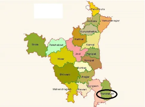
Faridabad located at 28.4211°N 77.3078°E in the South eastern part of Haryana has Gurugram and Palwal as its neighbouring districts. It has sub tropical climate with hot summers and cold winters. The area gets sufficientrainfall in the summer season and some rain in the winter season. The study area is depicted in Figure 1 [12].
Figure 1. Map of the Study Area
The parameters of the dataset include the AQI and the concentration of carbon monoxide (CO), sulphur dioxide (SO2), nitrogen dioxide (NO2), PM2.5 and ozone.
2.2 Mathematical Model for Computing AQI
The scheme that is used to convert the concentration of various air pollutants into a single value is called air quality index. It transforms the various parameter values of the pollutants into one value by the use of numerical manipulation. The process of computation of AQI consists of the following two steps:
a) Calculation of Sub- Index
The sub index Si for the concentration of pollutant Ai is calculated using a sub index function. The sub index signifies the relationship between the pollutant concentration and its corresponding health effect. The linear relationship between the sub index and the pollutant concentration is represented as follows:
Where m is the slope of the line and b is the intercept at A=0.
The general equation for the calculation of sub index Si given the pollutant concentration Ap is as follows:
Where,
Clo is the breakpoint concentration less than or the same as the given pollutant concentration.
Shi is the value of the AQI corresponding to Chi Slo is the value of the AQI corresponding to Clo
b) Formation of AQI
The sub indices of the various pollutants are combined in a simple additive form or weighted additive form: to calculate the overall air quality index S as follows:
For the calculation of AQI in India, a mathematical function consisting of the maximum operator is used:
The maximum operator is used as it not ambiguous. Further, the weighted sum cannot be found as the effects that combination of pollutants has on human health is not known [10].
3. Supervised Learning Techniques
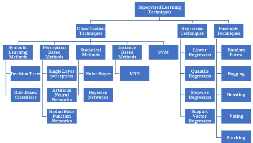
Supervised learning is learning that involves an expert that is well versed with the environment. In this type of learning, the response is found based on labelled training data. The desired response is given by the expert and the predicted response by the learning system [13]. The supervised learning techniques comprises of classification, regression and ensemble techniques where the target variable is categorical in classification and continuous in regression. Clustering is part of unsupervised learning [35, 36]. Ensemble techniques combine various models to increase the prediction accuracy. The existing classification, regression and ensemble techniques have been summarized in Figure 2.
3.1 Classification Techniques
Classification techniques play a major role to produce the general hypothesis to forecast the future data instances [30]. These techniques assign the class labels to the test dataset given the input predictors where the response is unknown [14,15].
Symbolic Learning methods perform prediction based on a set of rules. Decision trees and rule based classifiers are types of symbolic learning methods. Decision Trees perform classification by dividing the instances based on the values of the various parameters. Perceptron Based methods consists of classification algorithms that make predictions based on functions based on set of weights to be used with the input vector.Statistical methods perform classification by taking into account the probability of an instance. Naive Bayes is represented by directed acyclic graph with the independence between one parent node and many children nodes. Instance-based methods
postpone the induction till classification and use distance based metrics like k-Nearest Neighbors (kNN) [32]. Support Vector Machine (SVM) perform classification by using a hyperplane to separate the various classes. Both the sides of the hyperplane is called the margin [16].
3.2 Regression Techniques
Regression techniques are used to estimate the relationship between various predictor variables and the response variable. It is used when the response variable to be predicted has continuous values.
3.3 Ensemble Techniques
These methods combine various models to create a single aggregate model. Random Forest is constructed by merging the prediction made by a number of trees when each of the trees is trained independently and the result is found out by taking their average [21]. Bagging is an ensemble technique that performs classification by voting the class chosen by the majority of its base methods. AdaBoost is an algorithm based on boosting. It constructs each time a new training dataset based on the weights [22]. Stacking combines the predictions from different sub models using a base model [23]. The sub models can be constructed by using any classification or regression techniques [24].Majority Voting performs prediction by taking into consideration the maximum votes from various base models.
4. AQI Prediction Methodology
The air quality dataset including the parameters affecting AQI of Faridabad has been collected from Central Pollution Control Board (CPCB) website. The AQI is calculated from these parameters by calculating the sub index of each parameter and then applying the max operator using formula mentioned in Section 2. Noise/missing data has been ignored during pre-processing. Prediction has been carried out using various classification, regression and ensemble techniques. Further, the performance of these techniques has been evaluated based on various metrics. The AQI Prediction methodology has been depicted in Figure 3.
Figure 3. AQI Prediction Methodology
4.1 Air Quality Index Dataset
Figure 4. Subset of Air Quality Dataset
From the various parameters of the collected dataset, the sub index and the air quality index has been calculated using mathematical formula. Further, AQI has been converted to a categorical variable based on the National Ambient Air Quality Standards specified in Table 1.
Table 1. National Air Quality Index
Value of AQI Category of AQI
0-50 Good
51-100 Satisfactory
101-200 Moderately Polluted 201-300 Poor
301-400 Very Poor 401-500 Severe
4.2 Metrics used for AQI Prediction
The various parameters used for performance evaluation of the classification techniques are Precision, Recall, Accuracy, Error rate, F1 score and ROC curve [25, 28]. These parameters have been discussed as follows:
Table 2. Confusion Matrix for a Three Class Problem
Predicted
Observed
P Q R
P TP EPQ EPR
Q EQP TQ EQR
R ERP ERQ TR
True positive: Correctly predicted instances for each class True Negative: Correctly rejected instances for each class False Positive: Incorrectly predicted instances for each class
False Negative: Incorrectly rejected instances for each class
• Precision
It specifies given a class, the number of correctly predicted instances for all predicted labels [34]. It is defined by:
Where T and F are the number of true positive and false positive instances of a given class.
Given a 3 class confusion matrix, Precision for class P is defined as:
• Recall
Recall also called Sensitivity indicates the number of correctly predicted instances from all the instances that should have that class label Recall is defined as:
Where T and F’ are true positives and false negatives predictions for a particular class.
For the given 3 class confusion Matrix:
• Accuracy
It is defined as total correct predictions divided by the size of the dataset [33]. Accuracy is defined as:
Where N is the size of the dataset.
• Error Rate
Error rate is the ratio of total incorrect predictions and the size of the dataset. It is defined as:
• F1 Score
• Receiver Operating Characteristic (ROC) Curve It is a plot between true positive rate and false positive rate. Every point on the curve represents a recall and precision pair for a threshold value [27].
The various parameters used for performance evaluation of the regression techniques are correlation coefficient, coefficient of determination, min max accuracy and mean absolute percentage error [27].
• Correlation Coefficient
The measure of the linear or nonlinear relationship between the input and output variables is specified by the correlation coefficient. Its value ranges between +1 and -1. A negative correlation means that the response varies inversely with the predictor. A lower correlation value specifies that there is a need to add more predictor variables in order to explain the variation of the response. The Pearson correlation coefficient between predictor variables Qi and response variable Pi is calculated as:
Where Q’’ and P’’ are the mean values of predictor Q and response P respectively.
• Coefficient of Determination
It can be calculated by squaring the value of Pearson correlation coefficient. This parameter represents goodness of fit and lies between 0 and 1. It is specified as fraction of variation in response by the variation in predictor as specified by the linear relationship between them. The coefficient of determination is computed as:
Where P, P’ and P’’ are the observed, predicted and average value of response variable respectively.
• Min Max Accuracy
Min Max accuracy is a measure that calculates the average between the minimum and maximum prediction of the response variable. It is calculated as:
Where P and P’ are the observed and predicted value of response variable respectively.
• Mean Absolute Percentage Error (MAPE)
MAPE specifies the difference between the actual response
and predicted response in percentage. It is calculated as the average of the absolute error of response in percentage. It is given by:
Where n is the size of the dataset and P and P’ are the observed and predicted value of response variable respectively.
5. Results Analysis of Air Quality
Dataset
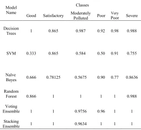
To predict the AQI, three classification techniques namely Decision tree, Naïve Bayes and SVM and three ensemble techniques namely Random Forest, Voting and Stacking have been used. Stacking ensemble has been performed by sub models: Decision Trees, SVM, Naïve Bayes and Random Forest with Logistic Regression as the base model. All the sub models used in stacking has been used to perform majority voting. The performance of these classification and ensemble techniques has been evaluated based on number of metrics. The results of Precision and Recall for each of the class label for each classification and ensemble technique has been depicted in Table 3 and Table 4 respectively.
Table 3. Precision Values for Various Classification and Ensemble Techniques
Model Name
Classes
Good Satisfactory ModeratelyPolluted Poor Poor Very Severe
Decision
Trees 1 0.865 0.987 0.92 0.98 0.988
SVM 0.333 0.865 0.584 0.50 0.91 0.755
Naïve
Bayes 0.666 0.78125 0.5675 0.90 0.77 0.8636
Random
Forest 0.866 1 1 1 1 0.988
Voting
Ensemble 1 1 0.9756 0.96 1 1
Stacking
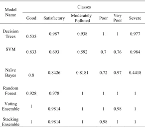
Table 4. Recall Values for Various Classification and Ensemble Techniques
From the above tables, it has been observed that ensemble techniques have higher values of precision and recall than classification techniques and Decision Trees have the highest of these values out of all the classification techniques. It is further observed that the lowest value of precision and recall exists for Support Vector Machines. Next, the accuracy, error rate and F1 score has been calculated for each classification and ensemble technique. To calculate the F1 score for each technique, the average precision and average recall for all classes has been taken into consideration. These results have been depicted in Table 5.
Table 5. Metrics Used for Performance Evaluation of Classification and Ensemble Techniques
From the above table, it has been observed that Decision Trees have the highest value of accuracy and F1 score among the classification techniques. Decision Trees have the lowest value of error rate. It is also observed that the values of lowest accuracy and F1 score exist for Support Vector Machine. The ensemble techniques observe higher accuracy and F1 score and lower error rate in comparison to the classification techniques. The Stacking ensemble has the highest value of accuracy and F1 score. The ROC curve for Random Forest is shown in Figure 5.
Figure 5. ROC Curve for Random Forest
In the above ROC curve, all the six classes have been depicted for the Random Forest technique. In the figure, the colours red, blue, yellow, green, black and magenta show the six classes Good, Satisfactory, Moderately Polluted, Poor, Very Poor and Severe respectively.
Further, prediction of AQI has been carried out using various regression techniques namely Linear Regression, Quantile Regression, Stepwise Regression and Support Vector Regression. The performance of regression techniques has been evaluated on metrics depicted in Table 6.
Table 6. Metrics Used for Performance Evaluation of Regression Techniques
Model Name
Classes
Good Satisfactory ModeratelyPolluted Poor Poor Very Severe
Decision
Trees 0.535 0.987 0.938 1 1 0.977
SVM 0.833 0.693 0.592 0.7 0.76 0.984
Naïve
Bayes 0.8 0.8426 0.8181 0.72 0.97 0.4418
Random
Forest 0.928 0.978 1 1 1 1
Voting
Ensemble 1 0.9814 1 1 0.98 1
Stacking
Ensemble 1 0.9814 1 0.98 1 1
Model Name Accuracy Error Rate F1 score
Decision
Trees 0.955 0.045 0.9315
SVM 0.743 0.257 0.7066
Naive Bayes 0.7393 0.2607 0.7352
Random
Forest 0.993 0.007 0.9799 Voting Ensemble 0.9914 0.0086 0.9922
Models r R2 Min/Max
Accuracy MAPE
Linear
Regression 0.96088 0.960883 78.519 0.312764
Quantile
Regression 0.96025 0.922087 82.330 0.206245
Stepwise
Regression 0.98644 0.973075 78.694 0.303793
Support Vector
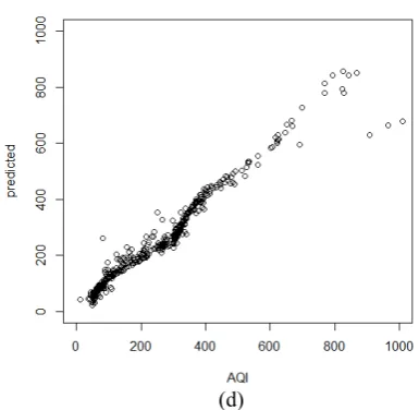
From the above table, it has been found that Support Vector Regression has the highest value of min max accuracy and least value of MAPE amongst all regression techniques. It is further found that Linear Regression has the lowest value of accuracy and highest value of MAPE. The plots between the predicted and the observed values of AQI have been depicted in Figure 6.
(a)
(b)
(c)
(d)
Figure 6. Predicted Vs Observed Values of AQI (a) Linear Regression (b) Quantile Regression (c)Stepwise Repression (d) Support Vector Regression
6. Conclusion
References
[1] Jasleen Kaur Sethi, Mamta Mittal (2018). A Study of Various Air Quality Prediction Models. Circulation in Computer Science, ICIC 2017, 128-131.
[2] Wang, D., Wei, S., Luo, H., Yue, C., & Grunder, O. (2017). A novel hybrid model for air quality index forecasting based on two-phase decomposition technique and modified extreme learning machine. Science of The Total Environment, 580, 719-733.
[3] Veljanovska, K., & Dimoski, (2018) A. Machine Learning Algorithms in Air Quality Index Prediction.
[4] Liu, B. C., Binaykia, A., Chang, P. C., Tiwari, M. K., & Tsao, C. C. (2017). Urban air quality forecasting based on multi-dimensional collaborative support vector regression (svr): A case study of beijing-tianjin-shijiazhuang. PloS one, 12(7), e0179763.
[5] Kumar, D. (2018). Evolving Differential evolution method with random forest for prediction of Air Pollution. Procedia computer science, 132, 824-833.
[6] Sharma, A., Mitra, A., Sharma, S., & Roy, S. (2018, October). Estimation of Air Quality Index from Seasonal Trends Using Deep Neural Network. In International Conference on Artificial Neural Networks (pp. 511-521). Springer, Cham.
[7] Saxena, A., & Shekhawat, S. (2017). Ambient air quality classification by grey wolf optimizer based support vector machine. Journal of environmental and public health, 2017.
[8] Lei, K. S., & Wan, F. (2012, July). Applying ensemble learning techniques to ANFIS for air pollution index prediction in Macau. In International Symposium on Neural Networks (pp. 509-516). Springer, Berlin, Heidelberg.
[9] Yu, R., Yang, Y., Yang, L., Han, G., & Move, O. (2016). RAQ–A random forest approach for predicting air quality in urban sensing systems. Sensors, 16(1), 86.
[10] https://timesofindia.indiatimes.com/city/delhi/14-of-
worlds-15-most-polluted-cities-in-india/articleshow/63993356.cms (accessed 30th March, 2019)
[11] Central Pollution Control Board (CPCB), Government of India. http://cpcb.nic.in/. (accessed 30th March, 2019)
[12] http://www.haryanaonline.in/ (accessed 30th March, 2019)
[13] Mittal, M., Goyal, L. M., Sethi, J. K., & Hemanth, D. J. (2019). Monitoring the Impact of Economic Crisis on Crime in India Using Machine Learning. Computational Economics, 53(4), 1467-1485.
[14] Mittal, M., Goyal, L. M., Hemanth, D. J., & Sethi, J.
K. Clustering approaches for high‐dimensional databases:
A review. Wiley Interdisciplinary Reviews: Data Mining and Knowledge Discovery, e1300.
[15] Nikam, S. S. (2015). A comparative study of classification techniques in data mining algorithms. Oriental journal of computer science & technology, 8(1), 13-19.
[16] Kotsiantis, S. B. (2007). Supervised Machine Learning: A Review of Classification Techniques. Informatica, 31, 249-268.
[17] Sánchez, A. S., Nieto, P. G., Fernández, P. R., del Coz Díaz, J. J., & Iglesias-Rodríguez, F. J. (2011). Application of an SVM-based regression model to the air quality study at local scale in the Avilés urban area (Spain). Mathematical and Computer Modelling, 54(5-6), 1453-1466.
[18] Koenker, R., & Hallock, K. F. (2001). Quantile regression. Journal of economic perspectives, 15(4), 143-156.
[19] Koenker, R. (2004). Quantile regression for longitudinal data. Journal of Multivariate Analysis, 91(1), 74-89.
[20] Lewis, M. (2007). Stepwise versus Hierarchical Regression: Pros and Cons. Online Submission.
[21] Denil, M., Matheson, D., & De Freitas, N. (2014, January). Narrowing the gap: Random forests in theory and in practice. In International conference on machine learning (pp. 665-673).
[22] Kotsiantis, S., & Pintelas, P. (2004). Combining bagging and boosting. International Journal of Computational Intelligence, 1(4), 324-333.
[23] Wang, G., Hao, J., Ma, J., & Jiang, H. (2011). A comparative assessment of ensemble learning for credit scoring. Expert systems with applications, 38(1), 223-230.
[24] Zhai, B., & Chen, J. (2018). Development of a stacked ensemble model for forecasting and analyzing daily average PM 2.5 concentrations in Beijing, China. Science of the Total Environment, 635, 644-658.
[26] Forman, G. (2003). An extensive empirical study of feature selection metrics for text classification. Journal of machine learning research, 3(Mar), 1289-1305.
[27] Gunawardana, A., & Shani, G. (2009). A survey of accuracy evaluation metrics of recommendation tasks. Journal of Machine Learning Research, 10(Dec), 2935-2962.
[28] Hemanth, D. J., Anitha, J., & Mittal, M. (2018). Diabetic retinopathy diagnosis from retinal images using modified hopfield neural network. Journal of medical systems, 42(12), 247.
[29] Dholakia, H. H., Purohit, P., Rao, S., & Garg, A. (2013). Impact of current policies on future air quality and health outcomes in Delhi, India. Atmospheric environment, 75, 241-248.
[30] Li, H., Wang, Y., Wang, H., & Zhou, B. (2017). Multi-window based ensemble learning for classification of imbalanced streaming data. World Wide Web, 20(6), 1507-1525.
[31] Huang, J., Peng, M., Wang, H., Cao, J., Gao, W., & Zhang, X. (2017). A probabilistic method for emerging topic tracking in microblog stream. World Wide Web, 20(2), 325-350.
[32] Zhang, J., Tao, X., & Wang, H. (2014). Outlier detection from large distributed databases. World Wide Web, 17(4), 539-568.
[33] Jiang, H., Zhou, R., Zhang, L., Wang, H., & Zhang, Y. (2018). Sentence level topic models for associated topics extraction. World Wide Web, 1-16.
[34] Peng, M., Zeng, G., Sun, Z., Huang, J., Wang, H., & Tian, G. (2018). Personalized app recommendation based on app permissions. World Wide Web, 21(1), 89-104.
[35]Mittal, M., Sharma, R. K., Singh, V. P., & Kumar, R. (2019). Adaptive Threshold Based Clustering: A Deterministic Partitioning Approach. International Journal of Information System Modeling and Design (IJISMD), 10(1), 42-59.