6. Idiosyncratic Risk and Returns: The Case
for a More Efficient Class of Estimators
MOHINDER PARKASH, Department of Accounting & Finance, School of
Business Administration, Oakland University, Rochester, MI48309, USA
RAJEEV SINGHAL, Department of Accounting & Finance, School of
Business Administration, Oakland University, Rochester, MI 48309, USA, Email: [email protected]
YUN (ELLEN) ZHU, Department of Accounting & Finance, School of
Business Administration, Oakland University, Rochester, MI 48309, USA.
ABSTRACT
Volatility is a key input into many important financial decisions. Therefore, accurateforecast of volatility plays animportant role in making these decisions. Typically, volatility is forecast using realized volatility computed from closing stock prices. Employing expectation of volatilitiessuch calculated, several papers find that expected idiosyncratic risk is positively associated with contemporaneous returns. Yang and Zhang [2000] show that estimators belonging to the class of range-based estimators are more efficient than the estimators derived only from closing prices. Using the more efficient range-based volatility estimates, we find no evidence to support the hypothesis that idiosyncratic risk explains returns.
KEYWORDS: Idiosyncratic Risk, Range-based volatility, Expected volatility, Risk-return relationship.
INTRODUCTION
Broadly, research in this stream of finance has explored two interconnected issues: the estimation of realized volatilities; and translating realized volatilities into expectations of future volatilities. Our paper adds to this debate by analyzing a sparsely-used (in finance) class of volatility estimators based on enhanced information than just close-to-close returns. The estimators we present belong to the class of range-based estimators which have been shown to be more efficient than the estimators based on closing prices[e.g., Garman and Klass 1980; Yang and Zhang 2000]. We employ two range-based estimators based on daily high, low, open, and close pricesto find that contrary to the evidence documented in recent papers, no relationship exists between idiosyncratic risk and stock returns.
The classical finance theory is based on the idea that risk is positively associated with future returns, and that the only risk that matters is the systematic risk, commonly represented by beta. For example, the Capital Asset Pricing Model (CAPM), a well-known asset pricing modelpredicts that the future return of a stock depends on the stock’s market beta. In CAPM, idiosyncratic risk ceases to matter because it can be diversified away.However, the assumption that investors are adequately diversified has faced challengesfrom several empirical and theoretical papers which argue that investors may remain under-diversified for a variety of reasons. Levy [1978] lists studies which show that individual investors are highly undiversified. More recently, Goetzmann and Kumar [2008] find that individual investors in the US are under-diversified and the level of under-diversification is higher for younger, low-income, educated, and less-sophisticated investors. These studies cast doubts about the notion that idiosyncratic risk is diversified away and should not be priced.
Our paper addresses two related issues—the impact of idiosyncratic risk on returns; and the measurement of idiosyncratic risk. To that end, we next present a review of the literature in the two areas. In the review, we first describe the research which shows that the use of a larger set of information than just closing prices yields more efficient estimatorsof realized volatilities. Second, we describe the state of theoretical and empirical research in the area of idiosyncratic risk and its effect on return.
MEASUREMENT OF VOLATILITIES
whether a more efficient estimator can be found by inclusion of more information than just the closing prices.
Garman and Klass [1980] is perhaps the earliest attempt at incorporating open, high, and low prices beside the close prices into estimation of volatilities. They show that the estimator derived using more information has a variance markedly lower than that of the classical estimator based on close-to-close prices. However, the Garman and Klass estimator is not independent of the drift and opening jumps in stock prices. To take into account drift in stock prices, Rogers and Satchell [1991] proposed a drift-independent model based on multiple price points during a trading day. But Rogers and Satchell [1991] corrects only for the drift and does not account for opening jumps.Yang and Zhang [2000] develop a minimum-variance estimator which is independent of both drift and opening jumps. In this paper, we use Rogers and Satchell [1991] and Yang and Zhang [2000] estimators of realized volatilities to conduct our analyses.
Idiosyncratic Risk and Returns
Mayers [1976] explores the effect of nonmarketable assets and market segmentation on assetprices. In his model, Mayers finds that under the assumption of constant relative risk aversion less than or equal to one, asset prices are lower given nonmarketable assets and market segmentation. In Mayers [1976] each investorholds a unique portfolio contrary to the prediction from CAPM. Levy [1978] allows investors to hold portfolios with some given number of securities. He finds that individual stock variance is important in his model. Merton [1987] models capital market equilibrium in an incomplete information setting and finds that less well-known stocks with fewer investors will tend to have larger expected returns and that expected returns depend on both the market risk and the total variance. Campbell, Lettau, Malkiel, and Xu [2001] list several arguments for the importance of idiosyncratic risk to expected returns. These arguments include: a lack of investor diversification from not following the approach recommended by financial theory or due to constraint imposed by compensation policy; investors may diversify by holding a portfolio of thirty stocks or fewer which depending on the volatility of individual stocks may not be adequate; arbitrageurs who exploit mispricing of individual securities are exposed to idiosyncratic risk; idiosyncratic volatility becomes important in event studies; and option price on a stock depends on total volatility of returns which is made up of volatilities attributable to both the market and to a specific firm. AndMalkiel and Xu [2006] present a model in which if a group of investors does not hold the market portfolio, remaining investors will also not be able to hold the market portfolio and idiosyncratic risk may become important.
corrects for problems in the statistical methods used in prior studies. In a recent paper, GSC show that average monthly stock variance is positively associated with higher returns in the subsequent month. Fu [2009] uses the exponential GARCH models to estimate expected idiosyncratic volatilities and finds a positive relationship between the conditional idiosyncratic volatilities and expected returns. Malkiel and Xu [2006] control for factors like size, book-to-market, and liquidity in conducting their analyses for US and Japanese equities to find that idiosyncratic volatility is more important than either the β, the systematic risk, or the size in explaining the cross-section of returns. Huang, Liu, Rhee, and Zhang [2010] also document a positive relationship between conditional idiosyncratic volatility and expected returns.
Estrada [2000] uses a database of 28 emerging economies and finds that idiosyncratic risk is significant in explaining the cross-section of returns. Harvey [2000] uses data from 47 different countries to construct 18 different measures of risk. He finds that collectively idiosyncratic risk is positive in explaining the cross-section of expected returns. Brockman, Schutte, and Yu [2009] examine the relationship across 44 countries from 1980 to 2007. They find a significantly positive relationship and attribute it to under-diversification. Lee, Ng, and Swaminathan [2009] obtain data for G-7 countries over the 1990 to 2000 time period and find a positive relationship between idiosyncratic volatility and expected returns.
Although the evidence in favor of a positive relationship between idiosyncratic risk and returns seems dominant, some papers document conflicting results. Longstaff [1989] observes a consistently negative but insignificant relationship between variance and returns for the overall period 1926-1985 and for the three sub-periods in which he divides his sample. Bali, Cakici, Yan, and Zhang [2005] re-examine the relationship between average stock volatility and future returns to conclude that the results in GSC were driven because of small stocks traded on the NASDAQ and that the GSC results disappear when market values are used as weights instead of equal weights to compute average volatility. And Wei and Zhang [2005] find that the results in GSC are driven mainly by the data in the 1990s as the relationship between idiosyncratic risk and future returns disappears when they extend the sample to 2002. Wei and Zhang also raise the possibility that combining equally-weighted average volatility with value-weighted average return may be behind the results reported in GSC. Bali and Cakici [2008] employ a portfolio approach and use various different measures of idiosyncratic volatility, alternative weighting schemes, different breakpoints for the construction of portfolios, and two different samples to find no robust relationship between idiosyncratic volatility and expected returns. Finally, Ang, Hodrick, Xing, and Zhang [2006] find that stocks with high idiosyncratic volatilities have low average returns, which is the opposite of that documented in GSC.
In the next section we describe the two methods used in our paper to measure realized volatilities which will be used to estimate conditional volatilities.
MEASURES OF REALIZED VOLATILITY
Fama-French Three Factor Method
In this approach, the idiosyncratic volatility for a stock in a monthis computed as the standard deviation of residuals from the regression of daily excess returns on the daily Fama-French[1993; 1996]three factors in that month. Ang, Hodrick, Xing, and Zhang [2006] and Fu [2009] use this approach. Thus in a given month, we run the following regression for each stocki for days 1 through n in that month,
MEASURES OF REALIZED VOLATILITY
impose the restriction of a minimum of 15 days in a month for which a stock must have both a return and a non-zero trading volume.3
In our cross-sectional regressions, we include several control variables. Fama and French [1992] show that the book-to-market ratio (BM) and firm size (ME) are useful in explaining cross-sectional returns. Jegadeesh and Titman [1993] demonstrate that buying past winners and selling past losers generates significantly positive returns over the horizons between three and twelve months. Following Fu [2009], for a stock in a month, we include the cumulative returns (CRET) in the six month period ending two monthsprior to the month as an explanatory variable. Consistent with Chordia, Subrahmanyam, and Anshuman [2001],to capture liquidity and its variability, we introduce the turnover ratio (TURN)defined as the natural log of the number of shares traded in a month divided by the number of shares outstanding expressed as percentage and the natural log of the variability of the turnover ratio, defined as the coefficient of variation of the turnover ratio (CVTURN), in our regressions. We impose a restriction of at least 18 observations in the computation of the two turnover related variables. Additionally, we follow Anderson and Dyl [2005] rule of thumb and adjust the NASDAQ volume down by 50 percent before 1997 and 38 percent after 1997 to address the effect of double-counting of trading volume for firms listed on that exchange.Finally, we include the systematic risk (BETA) of a stock in our cross-sectional return model.
RESULTS
In Table 1, we present the autocorrelations for the three methods of realized volatilities. The autocorrelations for each firm are computed at various lags and then averaged across the sample firms. VAFF, the realized volatility based on closing prices decays relatively more quickly over the first three lags and then very slowly for higher lags. The more efficient realized volatilities based on information about high, low, open, and close prices (VARS and VAYZ) decay more quickly for four lags and appears to be persistent for lags greater than four.
Table 1
Autocorrelations for the Three Realized Volatility Measures
Variable LAG1 LAG2 LAG3 LAG4 LAG5 LAG6 LAG7 LAG8 LAG9 LAG10 LAG11 LAG12 VAFF 0.33 0.27 0.25 0.19 0.18 0.17 0.15 0.14 0.15 0.12 0.10 0.12 VARS 0.45 0.35 0.29 0.23 0.21 0.19 0.17 0.17 0.16 0.15 0.12 0.13 VAYZ 0.39 0.30 0.26 0.20 0.19 0.17 0.15 0.15 0.15 0.13 0.10 0.11
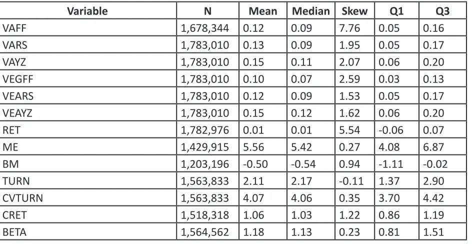
Table 2 describes our variables of interest. All the variables are winsorized at 0.5 percent in each tail. We also exclude observations with monthly returns of greater than 300 percent to minimize the possibility of recording errors contaminating our results. The mean and median realized volatilities using the range-based estimators (VARS and VAYZ) are higher than those using closing prices (VAFF). Mean and median volatility forecasts (VEGFF, VEARS, and VEAYZ) also show a similar pattern. Other variables are comparable to the numbers reported in Fu [2009] in terms of means and medians.VAFF and RET exhibit right skewness of more than 3, but the other variables do not appear to be highly skewed.
Table 2
Summary Sample Statistics
Variable N Mean Median Skew Q1 Q3
VAFF 1,678,344 0.12 0.09 7.76 0.05 0.16
VARS 1,783,010 0.13 0.09 1.95 0.05 0.17
VAYZ 1,783,010 0.15 0.11 2.07 0.06 0.20
VEGFF 1,783,010 0.10 0.07 2.59 0.03 0.13
VEARS 1,783,010 0.12 0.09 1.53 0.05 0.17
VEAYZ 1,783,010 0.15 0.12 1.62 0.06 0.20
RET 1,782,976 0.01 0.01 5.54 -0.06 0.07
ME 1,429,915 5.56 5.42 0.27 4.08 6.87
BM 1,203,196 -0.50 -0.54 0.94 -1.11 -0.02
TURN 1,563,833 2.11 2.17 -0.11 1.37 2.90
CVTURN 1,563,833 4.07 4.06 0.35 3.70 4.42
CRET 1,518,318 1.06 1.03 1.22 0.86 1.19
Sample correlations among our measures of realized volatilities, conditional volatilities, and returns contemporaneous with conditional volatilities are available in Table 3. Although realized volatilities are strongly correlated, the correlations between closing-price-based conditional volatility (VEGFF) and range-based volatilities (VEARS and VEAYZ) are relatively weaker. As expected, the two measures of range-based conditional volatilities are highly correlated. In the univariate analysis, the correlation between VEGFF and RET is insignificant, but significant and negative between VEARS and RET and VEAYZ and RET.
Table 3
Sample Correlations
Variable VAFF VARS VAYZ VEGFF VEARS VEAYZ RET
VAFF 1.00 0.77* 0.81* 0.28* 0.61* 0.62* -0.07*
VARS – 1.00 0.93* 0.31* 0.81* 0.79* -0.05*
VAYZ – – 1.00 0.29* 0.75* 0.76* -0.05*
VEGFF – – – 1.00 0.31* 0.31* 0.00
VEARS – – – – 1.00 0.94* -0.04*
VEAYZ – – – – – 1.00 -0.04*
RET – – – – – – 1.00
*Significant at the 1% level
In Table 4, we present our main result to test the hypothesis that there is a relationship between idiosyncratic risk and returns. In our cross-sectional regressions, the t-statistics are based on the Fama and MacBeth [1973] approach. Using all the sample firms, we run the cross-sectional regression with monthly stock returns as the dependent variable each month and generate a time series of monthly parameter estimates. From the time series of parameter estimates, we compute the mean estimate and the standard deviation of the estimate to calculate the t-value.
Table 4
Regression Results
BETA BM ME CRET TURN CVTURN VAFF VARS VAYZ VEGFF VEARS VEAYZ R2 (%)
0.005 0.001 0.000 – – – – – – – – – 3.5
(1.23) (1.88) (-0.21)
0.003 0.000 0.000 0.155 0.001 0.004 – – – – – – 17.7
(1.07) (-0.34) (0.03) (62.84) (1.04) (2.73)
0.004 -0.001 -0.002 0.153 0.002 0.006 -0.068 – – – – – 18.9
(1.61) (-2.04) (-4.24) (67.04) (2.11) (4.27) (-6.27)
0.003 -0.001 -0.001 0.153 0.001 0.004 – -0.014 – – – – 19.0
(1.20) (-1.36) (-1.48) (67.12) (2.14) (3.20) (-1.02)
0.003 -0.001 -0.001 0.153 0.001 0.004 – – -0.018 – – – 18.8
(1.28) (-1.31) (-2.11) (66.93) (1.83) (3.47) (-1.94)
0.002 0.000 0.000 0.155 0.001 0.004 – – – 0.013 – – 17.9
(0.90) (-0.11) (0.33) (63.43) (0.82) (2.62) (3.77)
0.003 0.000 0.000 0.155 0.001 0.004 – – – – 0.002 – 18.7
(1.03) (-0.22) (-0.13) (65.90) (1.14) (3.02) (0.12)
0.003 0.000 0.000 0.155 0.001 0.004 – – – – – 0.000 18.6
Numbers in bold are significant at better than 5% level
We present nine specifications of the return model. In the first specification, BETA, BM, and ME do not seem to be helpful in explaining returns. The explanatory power of the model given by r-square is also small (3.5 percent). We then introduce CRET, TURN, and CVTURN to the model. CRET and CVTURN are significant and the explanatory power of the model goes up to 17.71 percent.
Then we introduce our three measures of realized volatilities one by one into the return model with the seven exogenous variables. As in GSC, VAFF, VARS, and VAYZ are the naïve forecasts of conditional volatility.To wit, VARSrealized in the month t-1 is the forecast of conditional volatility in the month t.VAFF and VAYZ are negative at 5-percent level or better, VARS is not.
To get the main results of our paper, we finally include the three measures of conditional volatilities, VEGFF, VEARS, and VEAYZ. Consistent with Fu [2009] and Huang, Liu, Rhee and Zhang[2010], we find the closing-price-based volatility forecast, VEGFF, to be positive related to returns. However, the more precise measures of volatility, VEARS and VEAYZ are not significant in explaining returns and lead us to conclude that there is no relationship between idiosyncratic risk and returns.
CONCLUSION
based on closing stock prices and have been shown to be highly imprecise.We adopt two estimators of realized volatility from the class of range-based estimators shown to be much more efficient than the classical estimators and use them to forecast volatility. Contrary to recent papers, we find no evidence of a relationship between idiosyncratic risk and returns.
Our paper uses methodologies used in existing research to estimate conditional volatilities. Future research may explore the issue of relative merits of different methodologies used to forecast volatilities.
Notes
1 We get similar results if we choose the best-fit model using the Schwarz Bayesian criterion.
2 http://mba.tuck.dartmouth.edu/pages/faculty/ken.french/data_library.html
REFERENCES
1.Andersen, Torben G.,Tim Bollerslev, Francis X. Diebold, and Paul Labys, 2003, Modeling and Forecasting Realized Volatility, Econometrica 71, 579-625.
2.Anderson, Ann-Marie and Edward A. Dyl, 2005, Market Structure and Trading Volume, Journal of Financial Research 28, 115-131.
3.Ang, Andrew, Robert J. Hodrick, Yuhang Xing, and Xiaoyan Zhang, 2006, The Cross-Section of Volatility and Expected Returns, Journal of Finance 61, 259-299.
4.Bali, Turan and Nusret Cakici, 2008, Idiosyncratic Volatility and the Cross Section of Expected Returns, Journal of Financial and Quantitative Analysis 43, 29-58.
5.———., Nusret Cakici, Xuemin (Sterling)Yan, and Zhe Zhang, 2005, Does Idiosyncratic Risk Really Matter? Journal of Finance 60, 905-929.
6.Brockman, Paul, Maria G. Schutte, and Wayne Yu, 2009, Is Idiosyncratic Risk Priced: The International Evidence, Working paper, Lehigh University.
7.Campbell, John Y., Martin Lettau, Burton G. Malkiel, and Yexiao Xu, 2001, Have Individual Stocks Become More Volatile? An Empirical Exploration of Idiosyncratic Risk, Journal of Finance 56, 1-43.
8.Chordia, Tarun, Avanidhar Subrahmanyam, and V. Ravi Anshuman, 2001, Trading Activity and Expected Stock Returns, Journal of Financial Economics59, 3-32.
9.Estrada, Javier, 2000, The Cost of Equity in Emerging Markets: A Downside Risk Approach, Working paper, IESE Business School, Barcelona, Spain.
10.Fama, Eugene F. and Kenneth R. French, 1992, The Cross-Section of Expected Stock Returns, Journal of Finance47, 427-465.
11.———. and Kenneth R. French, 1996, Multifactor Explanations of Asset Pricing Anomalies, Journal of Finance 51, 55-84.
12.———. and James D. Macbeth, 1973, Risk, Return, and Equilibrium: Some Empirical Tests, Journal of Political Economy 81, 607-636.
13.French, Kenneth R., William Schwert, and Robert F. Stambaugh, 1987, Expected Stock Returns and Volatility, Journal of Financial Economics 19, 3-29.
14.Fu, Fangjian, 2009, Idiosyncratic Risk and the Cross-Section of Expected Stock Returns, Journal of Financial Economics 91, 24-37.
15.Garman, Mark B. and Michael J. Klass, 1980, On the Estimation of Security Price Volatilities from Historical Data, Journal of Business 53, 67-78.
17.Goyal, Amit and Pedro Santa-Clara, 2003, Idiosyncratic Risk Matters! Journal of Finance 58, 975-1007.
18.Harvey, Campbell R., 2000, The Drivers of Expected Returns in International Markets, Working paper, Duke University and National Bureau of Economic Research.
19,Huang, Wei, Qianqiu Liu, S. Ghon Rhee, and Liang Zhang, 2010, Return Reversals, Idiosyncratic Risk, and Expected Returns, Review of Financial Studies 23, 147-168.
20.Jegadeesh, Narsimhan, and Sheridan Titman, 1993, Returns to Buying Winners and Selling Losers: Implications for Stock Market Efficiency, Journal of Finance 48, 65-91.
21,Lee, Charles, David Ng, and Bhaskaran Swaminathan, 2009, Testing International Asset Pricing Models Using Implied Cost of Capital, Journal of Financial and Quantitative Analysis 44, 307-335.
22.Lehmann, Bruce N., 1990, Residual Risk Revisited, Journal of Econometrics 45, 71-97.
23.Levy, Haim, 1978, Equilibrium in an Imperfect Market: A Constraint on the Number of Securities in the Portfolio, American Economic Review 68, 643-658.
24.Longstaff, Francis A., 1989, Temporal Aggregation and the Continuous-Time Capital Asset Pricing Model, Journal of Finance 44, 871-887.
25.Malkiel, Burton G. and Yexiao Xu, 2006, Idiosyncratic Risk and Security Returns, Working paper, University of Texas at Dallas.
26.Mayers, David, 1976, Nonmarketable Assets, Market Segmentation, and the Level of Asset Prices, Journal of Financial and Quantitative Analysis 11, 1-12.
27.Merton, Robert C., 1987, A Simple Model of Capital Market Equilibrium with Incomplete Information, The Journal of Finance 42, 483–510.
28.Rogers, L. C. G., and Stephen E. Satchell, 1991, Estimating Variance from High, Low and Closing Prices, Annals of Applied Probability 1, 504–512.
29.———., Stephen. E. Satchell, andYoungjun Yoon, 1994, Estimating the Volatility of Stock Prices: A Comparison of Methods that Use High and Low Prices, Applied Financial Economics 4, 241–247.
30.Wei, Steven X. and Chu Zhang, 2005, Idiosyncratic Risk does not Matter: A Re-Examination of the Relationship between Average Returns and Average Volatilities, Journal of Banking and Finance 29, 603-621.