An Automated Method for Brain Tumor Segmentation Based on Level Set

(1)

An Automated Method for Brain Tumor Segmentation

Based on Level Set

Maryam Taghizadeh Dehkordi

*

Faculty of Technology and Engineering, Shahrekord University, Shahrekord, Iran

Email: [email protected]

Abstract

In this paper, an automatic method has been proposed for tumor segmentation. In this method, a new energy

function by introducing the feature tumor is determined implemented by level set. Multi-scale Morphology

Fuzzy filter is applied to the image and its output determines the tumor feature. The initial contour selection is

important in active contour models. Therefor the initial contour has been selected automatically by using Hough

transform and morphology function. Experimental results on MR images verify the desirable performance of the

proposed model in comparison with other methods.

Keywords: Tumor segmentation; Multi-scale fuzzy filter; feature; energy function; Level set.

1.Introduction

Based on the World Health Organization (WHO), nearly half thousand people suffer from brain tumor each

year. The tumors cloud be seen at different location with different intensities and differ in shape and size. As a

result, precise segmentation of brain tumors is a very challenging task beside its great interest. Fatality and the

rate of spread of tumors fall them into two major categories namely: Benign and malignant brain

tumors. Patients suspected of having tumors undergo many diagnostic CT-scans and MRI in hospitals. Tumor

identification is extremely hard due to some abnormalities and noise, as a result radiologist face with a

challenging operation. Numerous methods have been proposed in the field of tumor segmentation. Lee and his

colleagues [1] inspected the use of the support vector machine (SVM) classification method and Markov random

fields (MRFs) for brain tumor segmentation and claimed the advantage of SVM-based approach. In [2] by using

biologically inspired BWT and SVM, the MR images were analyzed for Brain Tumor Detection and Feature

Extraction. Tumor volume in MR images effectively measured by Fuzzy-correctness method [3,4].

---

(2)

Other common methods used in segmentation of many types of medical image processing are Convolutional

Neural Networks (CNNs) and region growing methods [5, 6]. Active Contour is one of the most popular methods

used in image segmentation. By minimizing of energy function, the curve stops on the true boundary of the target

object.

Active contour models are one of the most effective methods in segmentation of clinical images. Active contours

can be categorized as edge-based [7–9] or region-based [10–11]. In region-based models, the statistical

information inside and outside of the contour control its evolution. These models have more effective

performance in images with weak edges or no edges and are less sensitive to noise. Popular region-based active

contour models can segment images with the intensity homogeneity [10–11]. However, intensity inhomogeneity

often arises in real images like clinical images.

In magnetic resonance images, intensity inhomogeneity refers to the non-uniform magnetic fields caused by

limitations in imaging devices and variations in the object susceptibility. Intensity inhomogeneity must be

corrected to remove undesired effects in analysis of MR images.

In [12-16], region-based models were proposed to segment the images with intensity inhomogeneity. For

example, Li and his colleagues [12] and Zhang and his colleagues [14] proposed local binary fitting (LBF) and

local image fitting (LIF) models, respectively, to combat intensity inhomogeneity by embedding local intensity

information into their models. In [16], a novel level set method was proposed for segmentation these images.

In this paper, a new energy function is defined for tumor segmentation by using tumor feature. This energy

function is implemented by level set method. First, a multi-scale fuzzy filter is applied to the image. The proposed

filter output obtained in a multi-scale framework as tumor feature, determines the probability of each pixel

belonging to the tumor structure. This function forces the active contour to coincide with the boundaries of tumor,

more precisely. The active contours in [14, 16] have not this ability.

The remainder of this paper is organized as follows: In Section 2, first, we review the most popular region-based

active contour models then the proposed method for tumor feature segmentation is described. The experimental

results on MR images and discussion are presented and assessed in Section 3. Section 4 is devoted to conclusions.

2. Materials and Methods

2.1. Region -based active contour models

Mumford and Shah defined an optimal piecewise smooth approximation function u of a given initial image I, for

energy minimization problem. In practice, it is difficult to minimize the Mumford–Shah functional due to

different dimensions of u and contour and also the non-convexity of the functional.

Chan and Vese [10] proposed an active contour, CV model inspired by the Mumford–Shah model. Their

(3)

C

dxdy

c

y

x

I

dxdy

c

y

x

I

c

C

E

C out C in CV

µ

λ

+

−

+

−

=

∫∫

2 ) ( 2 2 2 ) ( 1 1 2 1

)

,

(

)

,

(

)

,

(

(1)

where λ1 and λ2 are positive constants, in (C) and out (C) represent the regions inside and outside the contour C,

respectively, c1 and c2 are two constants that approximate the image intensity in in (C) and out (C). Thus, in

images with intensity inhomogeneity the original image data is not the same with c1 and c2. Consequently, the CV

model is not applicable to such images.

In [12-15], region-based models were proposed to segment the images with intensity inhomogeneity. For

example, in [14] local fitted image (LIF) formulation was defined as follows:

)) ( 1 ( ) ( 2

1Hε φ m Hε φ

m

ILIF = + − (2)

where are defined as follow:

{







∩

>

Ω

∈

=

∩

<

Ω

∈

=

)))

(

}

0 )

(

)))

(

}

0 )

(

2 1

x

W

x

I

mean

m

x

W

x

I

mean

m

k k

φ

(3)

where Wk(x) is a rectangular window function, e.g. a truncated Gaussian window or a constant window. In this

experiment, a truncated Gaussian window _K_σ₍_x₎ with standard deviation

σ

and of size 4k+1 by 4k+1 was

chosen, where k is the greatest integer smaller than s. In [14] a local image fitting energy functional by

minimizing the difference between the fitted image and the original image was proposed. The formulation is as

follows:

Ω

∈

−

=

_∫

Ω

I

x

I

x

dx

x

E

LIF

(

)

LFI

(

)

,

2

1 )

(

φ

2 (4)

Using the calculus of variation and the steepest descent method [17],

E

LIF

(

φ

)

was minimized with respect to f

to get the Corresponding gradient descent flow:

)

(

)

)(

(

1 2

δ

φ

ε

m

I

t

LIF

−

=

∂

(5)

where

δ

_ε

(

φ

)

is the regularized Dirac function defined in Eq.(11).

In [16] The inhomogeneous objects are modeled as Gaussian distributions of different means and variances in

which a sliding window is used to map the original image into another domain, where the intensity distribution of

(4)

Moreover, since the models only extract local intensity means which are close to the background means in tumor

structure, it fails to detect tumors, carefully. Thus, to detect tumorsprecisely, more accurate characterization of

tumors is to be introduced to model as [18]. The goal of this paper is to relieve these drawbacks.

2.2. Determination of tumor features

The tumor tissue mainly appears in brighter colors than the rest of the regions in the brain and mass. Based on

these observations, we use a fuzzy Morphology filter to enhance tumor structure in MR images.

In the next, the definition of fuzzy morphology filter is presented, followed by the morphology operator to

extract local image information.

2.3. Fuzzy morphology filter

Given an universe U, a mapμX : U → [0, 1], x → μX (x) ∈[0, 1] defines a fuzzy set X on U. Many transfer

functions can be used to map an image F into a fuzzy set

F

′

. We use the membership function of the fuzzified

image that is calculated as:

min

max

min

)

,

(

)

,

(

F

n

m

F

n

m

F

−

=

′

(6)

Where F(m,n) is the pixel value at (m, n)th position. Fmin and Fmax are the maximum and minimum grey values of

the image, respectively. On the normalized image, fuzzy morphological erosion, dilation, opening, closing, and

top-hat of

F

′

by A are, respectively, defined as follows [19]:

)

,

(

F

A

E

A

F

′

⊕

=

′

)

,

1 (

1 E

F

A

F

′

Θ

=

−

′

)

),

,

(

1 (

1 E

E

F

A

F

′

o

=

−

′

)

),

,

(

1 (

E

F

A

E

A

F

′

• =

−

′

(7)

(8)

(9)

(10)

Fuzzy erosion can be computed by using different matrices. One of them is the average function

s

A

F

E

=

1 −

∑

′

−

/

(11)

where s is the number of active pixels in the SE. More detailed explanation about the fuzzy morphological

(5)

In order to obtain the feature of tumors with various sizes, the fuzzy opening acts applied at different scales in a

certain range.

The filter is analyzed at different scales SE in a range S. When the scale matches the size of the tumor, the filter

response will be maximum. Therefore, the final proposed filter response is

SE y x F y

x =SES ′ Θ

F( , ) max∈ ( , ) (12)

For each pixel (x,y), Φ(𝑥𝑥.𝑦𝑦) estimates the measure to be tumor using tumor features extracted by multiscale

fuzzy morphology analysis.

The result of the proposed filter for two MR images is shown in Fig.1.

Figure 1: The result of our filter on a MR image (a, c) original images (b, d) The result of our filters

2.4.Proposed active contour model

We define the following energy function of a contour C:

dy

dx

y

x

f

y

x

f

C

E

C

N I

T

=

∫∫

−

2

)

(

,

)

(

,

)

2

1 )

(

(13)

where N(C) define a narrow band around C, that caused the energy is only calculated in a neighborhood of C. fI is

the feature image defined as:







∈

=

)

(

)

,

(

,

)

(

)

,

(

,

)

,

(

2 1

C

outside

y

x

c

C

inside

y

x

c

y

x

f

_I (14)

For each pixel (x,y) , 𝑓𝑓_𝐼𝐼(𝑥𝑥.𝑦𝑦) approximates its intensity according to its feature. c1 and c2 of (7) can be viewed as

(6)

. ) , ( ) , ( )) , ( 1 )( , ( ) , ( , ) , ( ) , ( ) , ( ) , ( ) , ( ) ( ) ( ) ( ) ( 2 ) ( ) ( ) ( ) ( 1

∫ ∫

′ ′ ′ − ′ − ′ ′ ′ − ′ − ′ ′ − = ′ ′ ′ − ′ − ′ ′ ′ − ′ − ′ ′ = C output C N C output C N C input C N C input C N y d x d y y x x K y d x d y y x x K y x f y x f y x c y d x d y y x x K y d x d y y x x K y x f y x f y x c I I I I σ σ t σ σ t (15)

where K_σis the Gaussian function with standard deviation σ. The weights are adjusted by _f_t₍_x′_,_y′₎ to be high

inside the tumor, where the measure

F

(

x

′

,

y

′

)

is also high, and low otherwise.

)) ) , ( arctan( 2 1 ( 2 1 ) , (

t

π

t − ′ ′ F + = ′

′ y x y

x

f (16)

Therefore, in this model, the intensity for each pixel (x,y) is estimated by a weighted average of the pixel

intensities in a neighborhood around (x,y). These weights are controlled by f_τ and K_σ functions. Thus, if (x,y)

belongs to a tumor, c1 is high and c2 is low and if (x.y) belongs to background c1 is low and c2 is high. Thus, it

can successfully detect tumor in images with intensity inhomogeneity by using local information and tumor

features. The proposed energy function is implemented by the level set method described below.

2.5.Level set method

In level set methods, the curve

C

⊂

Ω

is represented by the zero level set of a Lipschitz function

φ

:

Ω

→

R

.

we propose to minimize the energy functional:

). ( ) ( ) ( )

(φ =λET φ +µρ φ +υϑφ

F (17)

The level set evolution equation for minimizing the energy functional (11) becomes:

) � � ( ) ( )) � � ( � ( ) )))( ( 1 ( ) ( -( )( ( ∂ ∂ 2 2 1 2 1

φ

δ

υ

φ

µ

φ

λ

φ

δ

φ

ε ε ε ε div div c c H c H c f t + − + − − + − = (18)

(7)

2 2 1 ) ( ) ( x x H x + = ′ = ε ε π

δε ε (19)

and c1 and c2 are calculated as:

. )) ( 1 )( ( )) ( 1 )( ( )) ( 1 )( ( ) ( , ) ( ) ( ) ( ) ( ) ( ) ( ) ( ) ( ) ( 2 ) ( ) ( 1

∫

− − − − = − = C N C N C N C N dy H y K dy H y x K y f y f x c dy H y K dy H y x K y f y f x c φ φ φ φ ε σ ε σ t ε σ ε σ t (20)

Here, _f_t₍_P₎ is calculated prior and c1, c2 and 𝑓𝑓_𝐼𝐼 are calculated iteratively.

2.6.Selection of initial contour

Initial contour selection is important in active contour models. The proper initial contour not only increases the

speed of convergence but the accuracy of segmentation. In this paper the initial contour is selected by combining

of Hough and morphology method. First the image is converted to binary, and then by using closing operator the

small objects are removed. According to that tumors are semi-circle, Hough transform imply to image and the

objects of circle is determined. As it is shown in fig.2, the algorithm can detect the tumor well from other areas of

the brain.

3. Results and Discussion

The proposed algorithm has been tested on MR images to evaluate the results of tumor detection. We used the

parameters

λ

=

1

,

µ

=

.

5

,

σ

=

2

,

t

=

0 .

1

,

t

=

0 .

1

as [13] respectively.

ε

=

1

in all experiments and for each case,

υ is chosen manually so that the best segmentation result is obtained. As shown in Fig.2, our method detects

tumors in images with inhomogeneity intensity and noise accurately. Another models extract part of background

as tumor.

(8)

In order to evaluate our method quantitatively, we randomly selected 21 MR images obtained in Hajar Hospital,

shahrekord, Iran. These images were segmented manually by an expert at this center as Gold standard.

To compare the performances quantitatively, we used true positive fraction (TPF) and false positive fraction

(FPF) indices. TPF, also called ‘sensitivity’, is the ratio of the number of pixels correctly classified as tumor

(TP), to the total number of tumor pixels in the gold standard segmentation

y sensitivit FN

TP TP P

TP

TPF =

+ =

= (21)

where FN is the number of pixels incorrectly classified as non-tumor. The ideal TPF is 1. FPF is the number of

pixels incorrectly classified as tumor (FP), divided by the total number of non-tumor pixels in the gold standard

y specificit TN

FP FP N

FP

FPF = −

+ =

= 1 (22)

Here, TN is the number of pixels correctly classified as non-tumor pixels. The ideal FPF is 0. The accuracy

(ACC) for one image is the ratio of the total number of correctly classified pixels (the sum of true positives and

true negatives) to the total number of pixels in the image

TN FP FN TP

TN TP N

P TN TP ACC

+ + +

+ =

+ +

= (23)

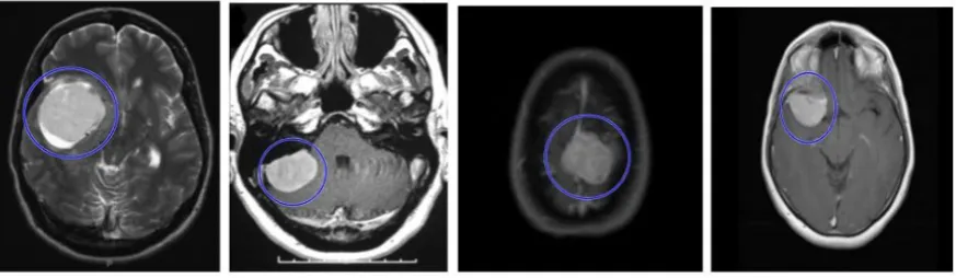
The ideal ACC is also 1. In Fig.3 (column a) three MR images are shown. The results of CV, LIF, the method in

[16] and the proposed method are shown in Fig.3(column b), (column c) , (column d) and ((column e),

respectively.

(9)

Images. Column (b) the results by CV. Column (c) the results by LIF. Column (d) the results by [16]. Column

(e) the results by the proposed method.

As shown in Fig. 3b, the CV model is able to extract the tumor, but a part of background is segmented as tumor.

The results of LIF and the method in [16] are shown in Fig. 3 (c, d), respectively. It is clear that the methods

cannot extract the tumors in images with a complex background accurately. According to Fig3, the great

performance of the proposed model in comparison with other methods is obvious.

To evaluate our method quantitatively, we selected 21 MR images from 21 patients obtained from Hajar

Hospital, Shahrekord, Iran. One expert at this center segmented these images as ground truth manually. Table 1

shows the average of the accuracy measurements for all 21 images with the proposed method, CV, LIF and the

model in [16]. It is apparent that our method outperforms other models in tumor segmentation. For example, it

exhibits a very low false positive error, which is very important in medical image segmentation.

Table1: Performance of tumor detection by the proposed active contour

4. Conclusion

In this paper, a new active contour model was proposed by introducing the tumor feature into its energy function

for tumor detection on 2-D MR images. The features were determined by applying a multi-scale morphology

fuzzy filter. The feature determines the probability of each pixel belonging to the tumor structure. For increasing

the speed of convergence and accuracy of segmentation, the initial contour is selected by combining of Hough

and morphology method. According to the results, this method is able to detect tumors in images with intensity

inhomogeneity and noise, correctly. The proposed method is a more accurate candidate for segmentation of brain

tumor in clinical tasks .

Acknowledgment

The authors wish to thank Hajar Hospital Doctors, for providing the images and manually segmenting tumors.

5.Conflict of Interest

There is no conflict of interest regarding the publication of this paper.

References

(10)

Pseudo Conditional Random Fields.” Med Image Comput Comput Assist Interv., vol.11, pp. 359-66.

2008.

[2] N. Bh Bahadure, A. K. Ray, and H. P. Thethi, “Image Analysis for MRI Based Brain Tumor Detection

and Feature Extraction Using Biologically Inspired BWT and SVM.” International journal of

Biomedical Imaging Vol. 2017, ID. 9749108, 2017

[3] J. Liu , J.K. Udupa , D. Odhner , D. Hackney , G. Moonis , “A system for brain tumor volume

estimation via MR imaging and fuzzy connectedness,” Comput Med Imaging Graph., vol. 29, no.1, pp.

21-34, Jan 2005.

[4] G.Moonisa, J.Liub, J.K.Udupab and D.B.Hackneya, “Estimation of Tumor Volume with

Fuzzy-Connectedness Segmentation of MR Images. ” American journal of neuroradiology, Vol.38, no.2,

2001.

[5] L.Zhao and K.Jia. “Multiscale CNNs for Brain Tumor Segmentation and Diagnosis,” Computational

and Mathematical Methods in Medicine, Vol. 2016 , Article ID 8356294, 2016

[6] T.Weglinski and A.Fabijanska, “Brain tumor segmentation from MRI data sets using region growing

approach, ” in Proceedings of the 7th International Conference on Perspective Technologies and

Methods in MEMS Design (MEMSTECH '11), pp. 185–188, May 2011.

[7] V. Caselles, R. Kimmel, and G. Sapiro, “Geodesic active contours,” Int. J. Comput.Vis, vol. 22, pp. 61–

79, 1997.

[8] Y. Xiang, A.C.S Chung, J. Ye, “An active contour model for image segmentation based on elastic

interaction.” Journal of Computational Physics, pp. 455–476, 2006.

[9] N. Paragios and R. Deriche, “Geodesic active regions and level set methods for supervised texture

segmentation.” Int. J. Computer.Vis., vol.46, pp. 223–247, 2002.

[10] T. Chan and L. Vese, “Active contours without edges.” IEEE Trans.Image Process., vol. 10, no. 2, pp.

266–277, Feb. 2001.

[11] X. Xie, M. Mirmehdi, “MAC: Magnetostatic Active Contour Model.” IEEE Tran.Pat.Ana, vol.30,

no.4, april 2008.

[12] C. Li, C.Y. Kao, J.C. Gore and Z. Ding, “Minimization of region-scalable fitting energy for image

segmentation.” IEEE Trans. Image Process., 2008, 17, (10), pp. 1940–1949

[13] M.T. Dehkordi, A. Doosthoseini, S. Sadri, and H. Soltanianzadeh, “local feature fitting active contour

(11)

[14] K. Zhang, H. Song and L. Zhang, “Active contours driven by local image fitting energy”, Patt.

Recognit., 2010, 43, pp. 1199–1206M.

[15] M. T. Dehkordi, M. Jalalat, S. Sadri, A. Doosthoseini, M. Ahmadzadeh, and R. Amirfattahi,

“Vesselness-guided Active Contour: A Coronary Vessel Extraction Method.” J Med Signals Sens.,

vol.4, no. 2, pp.150–157, Apr-Jun 2014.

[16] K. Zhang, L. Zhang, K. M. Lam, and D. Zhang, “A Level Set Approach to Image Segmentation With

Intensity Inhomogeneity.” IEEE transactions on cybernetcs, V0l.46. no.2, pp.546-57, 2016 Feb

[17] T. Lindeberg, “Scale-Space Theory in Computer Vision.” Kluwer Academic, Dordrecht, The

Netherlands, 1994

[18] M. T. Dehkordi, “A new active contour model for tumor segmentation.” 3rd International Conference

on Pattern Recognition and Image Analysis (IPRIA2017), pp.233-236.

[19] K. Sun, Zh. Chen, Sh. Jiang and Yu. Wang, “Morphological Multiscale Enhancement Fuzzy Filter and

Watershed for Vascular Tree Extraction in Angiogram.” Journal of Medical Systems