A time expanded version of the (Hitchcock-) transportation problem

(1)

DOI 10.1007/s12544-011-0056-3

ORIGINAL PAPER

A time expanded version of the (Hitchcock-)

transportation problem

Raffaele Mosca

Received: 27 January 2011 / Accepted: 7 September 2011 / Published online: 1 October 2011 © The Author(s) 2011. This article is published with open access at Springerlink.com

Abstract This paper considers a time expanded version of the classical (Hitchcock-) transportation problem. Certain quantities of goods are produced in the produc-tion facilities in each period of a planning horizon and also the demand values of the outlets are different for each time period. Moreover, the transportation costs fromito jalso vary over time. The different planning periods are connected by the fact that goods may be stored at a facility or at an outlet to exploit cheaper transportation costs as long as the demand is met in every time period. We describe the problem by two models, showing that it can be solved in polynomial time by standard software packages. Then we describe some generalizations of the problem by adapting the two models, pointing out that each model seems to provide different benefits.

Keywords Transportation problems· Min-cost flow problem·Hitchcock problem

1 Introduction

For notation and standard terminology, let us refer to [10] (see also [6,9]).

The (Hitchcock-) transportation problem is a well known problem in operations research [6,9,10] and can

R. Mosca (

_B

)

Dipartimento di Scienze,

Universitá degli Studi “G. d’Annunzio”, Pescara 65127, Italy

e-mail: [email protected]

be solved in polynomial time by fast algorithms (see e.g. [12]). By its applicative nature, several versions of this problem have been considered, such as dynamic, time-dependent versions (see e.g. [5]).

In this paper we consider a time expanded version, which is defined below as problem P. Problem Pwas studied in [2] (see also [3,4]) by referring to a method for solving integer programming which resorts to the calculation of suitable Gröbner bases [7]: in partic-ular, the authors call it 3-dimensional transportation problem (referring to [11], while a similar name was used in [1] for a different problem). The motivation of this paper is to try to study problem P by an op-erations research approach. The closest reference in this sense seems to be [8], where the authors study the existence of feasible solutions in a multiperiod allocation problem of substitutable resources: in par-ticular, at a certain point of the paper the authors call it a multiperiod transportation problem a prob-lem which however seems to be quite distant from problemP.

Let P be the following problem: Given r produc-tion facilities F1, . . . ,Fr, let Aik (i=1, . . . ,r, andk=

1, . . . ,t) denote the number of units of an indivisi-ble good produced by Fi during the k-th period of a planning horizon of t periods. Assume that there are s outlets O1, . . . ,Os each one demanding a certain

(2)

One can assume that the following conditions (1) and (2) hold true (as discussed below).

i=1,...,r

k=1,...,t¯

Aik≥

j=1,...,s

k=1,...,¯t

Bjk, fort¯=1, . . . ,t (1)

i=1,...,r

k=1,...,t

Aik=

j=1,...,s

k=1,...,t

Bjk (2)

If Eq.1 is not true, then the problem has no feasible solution (demand exceeds supply at the¯t-th period). If Eq.2is not true, then one may proceed similarly to the Hitchcock problem (i.e., problemPfort=1) as shown in [10] since all the costs are nonnegative: one may add, for k=1, . . . ,t, a fictitious outlet Ouk (with u=s+

1) and define Buk=

i=1,...,rAik−

j=1,...,sBjk, and ciuk=0 for i=1, . . . ,r; then define h_uk=0 for k=

1, . . . ,t.

Let us denote as:

• xijkthe amount of good which is sent fromFitoOj in thek-th period;

• zikthe amount of good which is stored in Fiat the end of thek-th period;

• z_jkthe amount of good which is stored inOjat the end of thek-th period.

A solution of P is determined by the values of xijk, zik,z_jk for i=1, . . . ,r,j=1, . . . ,s,k=1, . . . ,t: then let [xijk,zik,z_jk] denote a solution of P and C[xijk, zik,z_jk]denote its cost.

In this paper we propose two models forP: the first (Section2) is a natural min-cost flow model, while the second (Section3) is a Hitchcock model obtained by exploiting some peculiarities of the problem. Then we describe some possible generalizations ofPby adapting the two proposed models (Section4), pointing out that each model seems to provide different benefits.

2 A min-cost flow model forP

A network N = (σ, τ,V,E, w,c) is a digraph (V,E) together with a sourceσ ∈V with 0 indegree, with a terminalτ ∈Vwith 0 outdegree, with an edge-capacity functionw:E−→R, and with an edge-cost function c: E−→R. A flow f in N is a vector in R|E| _(one component f(u, v)for each(u, v)∈ E)such that:

(i) 0≤ f(u, v)≤w(u, v)for all(u, v)∈ E

(ii) ₍_u_,v)_∈_E f(u, v)=_(v,_u₎_∈_E f(v,u)for allv∈V\

{σ, τ}.

The value of fis the quantity:_(σ,_y₎_∈_E f(σ,y). The cost of f is the quantity:₍_u_,v)_∈_Ec(u, v)f(u, v).

Given a network N and a flow-value vf, the min-cost flow problem with respect to pair(N, vf)is that of computing inNa flow fof valuevf that has minimum cost.

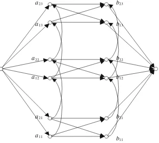
In the sequel, let us try to modelPas a min-cost flow problem in the following network, which is constructed by considering that Pimplicitly containstinstances of the Hitchcock problem and by adding an origin vertex, a destination vertex, and edges for the links between consecutive periods (see Fig.1):

• constructtdisjoint digraphsG1, . . . ,Gtsuch that:

Gk=(Vk,Ek),fork=1, . . . ,t, where

Vk= {aik:i=1, . . . ,r} ∪ {bjk: j=1. . . ,s}; Ek= {(aik,bjk):i=1, . . . ,r,j=1, . . . ,s};

Comment:vertexaikrepresents Fiat periodk, for

i=1, . . . ,r,k=1, . . . ,t; vertex bik represents Oj at the periodk, for j=1, . . . ,s,k=1, . . . ,t; edge (aik,bjk)represents the possibility of transporting good from Fi to Oj at period k, for i=1, . . . ,r,

j=1, . . . ,s,k=1, . . . ,t.

• add vertex σ and edges {(σ,aik):i=1, . . . ,r, k=1, . . . ,t};

• add vertex τ and edges {(bjk, τ): j=1, . . . ,s, k=1, . . . ,t};

• add edges{(aik,aik+1):i=1,. . .,r,k=1,. . .,t−1}; • add edges{(bjk,bjk+1): j=1, . . . ,s,k=1,. . .,t−1}; • the elements ofVandEare defined as above;

• the function w:E−→R of edge-capacities is defined as follows:

w((σ,aik))= Aik, fori=1, . . . ,r,k=1, . . . ,t; w((bjk, τ))=Bjk, for j=1, . . . ,s,k=1, . . . ,t; w(e)= ∞, for the remaining elementse∈E;

• the functionc: E−→Rof edge-costs is defined as follows:

c((aik,bjk))=cijk, for i=1, . . . ,r,j=1. . . ,s, k=1, . . . ,t;

c((aik,aik₊1))=hik, fori=1, . . . ,r,k=1, . . . ,t−1;

c((bik,bik+1))=hik, for j=1, . . . ,s,k=1, . . . ,t−1;

c(e)=0, for the remaining elementse∈ E. Let N= (σ, τ,V,E, w,c) be the network defined as above. By Eq. 1 it is possible to define in N a flow of valuevf =

j=1,...,r

(3)

Fig. 1 A min-cost flow model forPin the caser=2,s=2,

t=3

a

23

a

13

a

22

a

12

a

21

a

11

b

23

b

13

b

22

b

12

b

21

b

11

By Eq.1and by the structure of N, given a feasible solution [xijk,zik,z_jk] of P one can derive a feasible solution[y(u, v)]ofPf, and vice-versa, by the following equalities:

• xijk=y(aik,bjk) for i=1, . . . ,r,j=1, . . . ,s,k=

1, . . . ,t;

• zik=y(aik,aik+1)fori=1, . . . ,r,k=1, . . . ,t; • z_jk =y(bjk,bjk+1)for j=1, . . . ,s,k=1, . . . ,t.

Furthermore C[xijk,zik,z_jk] = ₍_u_,v)_∈_Ec(u, v)y(u, v), by the definition of costs for edges ofN.

One can formalize what above by the following theorem.

Theorem 1 An instance of P can be solved as a min-cost f low problem.

As network N can be efficiently constructed, one obtains the following corollary.

Corollary 1 Problem P can be solved in polynomial time.

In particular the problem admits an optimal integer solution if all the valuesAik,Bjkare integer.

3 A Hitchcock model forP

Let us consider problem P as problem Pf defined in Section2, according to the equalities linking the respec-tive solutions. In [10] a standard transformation from an instance of the min-cost flow problem to an instance of the Hitchcock problem is shown. However, in the sequel let us try to modelPas a Hitchcock problem just by exploiting some peculiarities of the problem (i.e., by compacting some aspects of Pf) and not by using the standard transformation of [10].

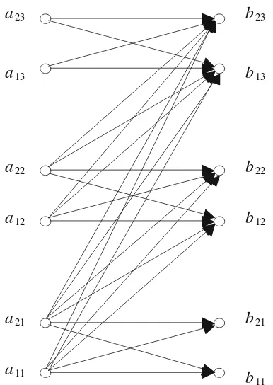
The Hitchcock model forPis based on the following variables (see Fig.2):

qiijj =the amount of good produced inFiat periodi,

and sold inOjat periodj.

Then (also by conditions (1) and (2)) one has:

qiijj≥0, (withqiijj =0, fori> j); (3)

j=1,...,s

j₌₁_,...,t

qiijj =Aii, fori=1, . . . ,r,i=1, . . . ,t;

(4)

i=1,...,r

i=1,...,t

qiijj=Bjj, for j=1, . . . ,s, j=1, . . . ,t.

(4)

a

23

a

13

a

22

a

12

a

21

a

11

b

23

b

13

b

22

b

12

b

21

b

11

Fig. 2 A Hitchcock model for Pin the caser=2,s=2,t=3

(the edges, i.e. the variables, withi> jare omitted)

It remains to define the costscii_jj.

Assume thati> j. Then one can defineciijj = ∞, so to ensureqiijj =0fori> j.

Assume thati≤ j.

Let us observe that for any solution ofP, the amount qiijjwill arrive fromFitoOjthrough a path fromaiito bjj in the networkNof Section2: in particular, all the edge-capacities along each of such paths are∞.

It follows that for any optimal solution of P, the amountqiijj will arrive fromFi to Ojthrough a least cost path (or in general through least cost paths, if more than one) fromaiitobjjin the networkNof Section2.

Then the cost cii_jj may be defined as the cost of a least cost path fromaii to bjj: by the structure of N such paths are exactly j−i+1(i.e., each such path is formed by a possible storage multi period in Fi, by a transfer period fromFitoOj, and by a possible storage multi period inOj: the transfer period is a periodkwith i≤k≤ j).

Then summarizing one obtains:

• ciijj= ∞, fori> j;

• ciijj= mini≤k≤j{(

u=i,...,k−1hiu)+cijk+(

u=k,...,j hju)}, fori≤ j.

Then the objective function_i₌₁_,...,_r_i₌₁_,...,_t_j₌₁_,...,_s

j=1,...,tciijjqiijjand the constraints (3), (4), (5) define

an instance of the Hitchcock problem (all the costs are non-negative), sayH.

Let us show that given an optimal solution [xijk, zik,z_jk]of Pone can derive a feasible solution [qiijj] ofH, and vice-versa.

From P to H Let [xijk,zik,z_jk] be an optimal solution

ofP. Then a solution [qiijj] ofHwith the same cost can be obtained as follows. Let us observe that: (i) the costs of storage in facilities (in outlet) do not depend on the destination (on the origin) of the good. By (i) and by the definition of costsciijj, one may proceed as follows. The first step may be to obtain the values of qikjk, for k=1, . . . ,t: to this end, for k=1, . . . ,t, it is enough to chose the values ofqikjk, in order to maxi-mize_i₌₁_,...,_r_j₌₁_,...,_sqikjk, subject toqikjk≤xijkand to

j=1,...,sqikjk≤ Aikfori=1, . . . ,r(that is to charge the values ofxijkto those ofqikjkas much as possible). That can be easily done by a greedy technique.

The second step may be to obtain the other values of qiijj: to this end one can apply the Ford–Fulkerson pro-cedure to compute a maximum flow in the network N obtained from the networkNof Section2by modifying the edge-capacities as follows:

• w((σ,aik))= Aik−

j=1,...,sqikjk , for i=1, . . . ,r, k=1, . . . ,t;

• w((bjk, τ))=Bjk−i=1,...,rqikjk , for j=1, . . . ,s, k=1, . . . ,t;

• w((aik,aik+1))=zik, fori=1, . . . ,r,k=1, . . . ,t;

• w((bik,bik+1))=zjk, for j=1, . . . ,s,k=1, . . . ,t;

• w((aik,bik))=xijk−qikjk , for i=1, . . . ,r,j=

1, . . . ,s,k=1, . . . ,t.

In fact, by starting from a null flow in N, at each iteration of the procedure an augmenting flow saturates a path in N from a certain lowest aii to a certain

highestbjj, withi< j (because of the first step): the value of such an augmenting flow can be charged onto qiijj, which may be updated at each iteration. Note that: concerning the cost, [qiijj] has the same cost as

[xijk,zik,z_jk], since the latter is an optimal solution of P and by the definition of costs ciijj; concerning the procedure, at mostt×(r×t)×(s×t)iterations occur, where the first t stands for an upper bound to the number of all possible paths fromaii tobjj.

From H to P Let [qiijj] be a solution of H. Then

a solution [xijk,zik,z_jk] of P with the same cost can be obtained as follows. By the definition of costsciijj,

(5)

the edges of Piijj, so to compose the values of a

so-lution [xijk,zik,z_jk] of Paccording to the equalities of Section2.

One can formalize what above by the following theorem.

Theorem 2 An instance of P can be solved (directly) as a Hitchcock problem.

Then a corollary and a comment similar to those at the end of Section2hold.

4 Some generalizations ofP

In this section let us introduce three possible general-izations of problemP, pointing out the advantages and the disadvantage of the two proposed models.

Let P1 be the following problem. In the context of

problemP, assume that every facilityFifori=1, . . . ,r (that every outletOjfor j=1, . . . ,s) can store at most di(at mostdj) units of good at the end of each period k for k=1, . . . ,t. The objective remains that of the problemP.

ThenP1can be modeled by the min-cost flow model

of Section2, by modifying the networkNas follows:

• w((aik,aik₊1))=di, fori=1, . . . ,r,k=1, . . . ,t; • w((bjk,bjk+1))=dj, forj=1, . . . ,s,k=1, . . . ,t.

ThenP1can be solved as a min-cost flow problem, i.e.,

in polynomial time.

On the other hand, it seems to be not immediate to modelP1by the Hitchcock model of Section3.

Let P2 be the following problem. In the context of

problemP, assume that the good produced in a facility has to be sold in a outlet before a certain number of periods (e.g., before corruption of the good), say L periods. The objective remains that of the problemP.

of Section2, by adding the following constraints:

• i=1,...,rzik+

j=1,...,szjk≤

¯

k=k,...,k∗Bjk¯ , fork=

1, . . . ,t, wherek∗=min{k+L,s}.

Actually in this way one obtains a generalization of the min-cost flow problem, which remains a linear pro-gramming problem, but can not be solved as a classical min-cost flow problem.

ThenP2can be modeled by the Hitchcock model of

Section3, by modifying the costs as follows:

• ciijj= ∞, for j−i>L,

so to ensureqiijj =0for j−i>L.

Then P2can be solved as a Hitchcock problem, i.e.,

in polynomial time.

Let P3 be the following problem: In the context

of problem P, letcik(i=1, . . . ,r,k=1, . . . ,t) be the cost of production for a unit of good in Fi in the k -th period, and let pjk(j=1, . . . ,s,k=1, . . . ,t) be the profit for selling a unit of good inOjin thek-th period: in particular, Aikcan be view as the maximum amount which can be produced by Fiin the k-th period. Then one wishes to minimize the total cost of transportation, of storage, and of production, less the total profit by selling, along the horizon oftperiods, i.e., one wishes to maximize the total profit by selling, less the total cost of transportation, of storage, and of production, along the horizon oftperiods.

A possible scenario for problem P3 may be that

of a tobacco manufacture company: in fact the selling price of tobacco varies over countries and its fluctuation (over countries) is planned in advance.

of Section2, by modifying the networkNas follows:

• c((σ,aik))=cik, fori=1, . . . ,r,k=1, . . . ,t;

• c((σ,bjk))= −pjk, forj=1, . . . ,s,k=1, . . . ,t.

Actually in this way one obtains a generalization of the min-cost flow problem (where: the costs are allowed to be negative, and the flow value is not fixed), which remains a linear programming problem, but can not be solved as a classical min-cost flow problem.

Then P3can be modeled by the Hitchcock model of

Section3as follows.

Let us observe that (recalling the definition of costs ciijj of Section3) it is possible and convenient to send good fromaii tobjjif and only if:

• i≤ j(it is possible);

• cii+mini_≤k≤j{(_u₌_i_,...,k−1hiu) +cijk + (

u=k,...,j

hju)} −pjj<0(it is convenient).

Let us say that a variableqiijjisgreenif the above two

conditions are satisfied.

For any green variableqiijj let us writec¯iijj=cii+ mini≤k≤j{(

u=i,...,k−1hiu)+cijk+(

u=k,...,jhju)}−pjj, and letKbe a scalar withK>|¯ciijj|.

Then let us define the following costsc∗_iijj for every

variableqiijj:

• c∗_iijj =K− |¯ciijj|, ifqiijjis a green variable;

• c∗_ii_jj =K, otherwise.

Let P∗₃ denote the Hitchcock problem (with all non-negative costs) defined by the objective function

i=1,...,r

i=1,...,t

j=1,...,s

(6)

Then it is not difficult to verify that, given an optimal solution [q∗_iijj] ofP∗3, one can directly derive an optimal

solution [qiijj] ofP3by setting:

• qiijj =q∗iijj , ifqiijj is a green variable;

• qiijj =0, otherwise.

ThenP3 can be solved as a Hitchcock problem, i.e., in

polynomial time.

Then summarizing it seems that: the first model is more powerful than the second model to describe gen-eralizations ofP(e.g.,P1), though it may lead to linear

programming which can not be solved as a classical min-cost flow problem (e.g., P2 and P3); while the

second model may be more useful than the first model to show that certain generalizations of P(e.g., P2 and

P3) can be solved as a classical Hitchcock problem.

5 Conclusions

The (Hitchcock-) transportation problem is a well known problem in operations research [6,9,10] and can be solved in polynomial time by fast algorithms (see e.g. [12]). By its applicative nature, several versions of this problem have been considered, such as dynamic, time-dependent versions (see e.g. [5]).

In particular the following time dependent version was studied in [2] (see also [3, 4]) by referring to a method for solving integer programming which resorts to the calculation of suitable Gröbner bases [7]:

Givenrproduction facilities F1, . . . ,Fr, let Aik(i=

1, . . . ,r, andk=1, . . . ,t)denote the number of units of an indivisible good produced by Fi during thek-th period of a planning horizon oftperiods. Assume that there aresoutlets O1, . . . ,Os each one demanding a

certain number of units per period, sayBjk(j=1, . . . ,s and k:=1, . . . ,t). Let cijk≥0 be the cost associated with transporting one unit fromFito Ojduring thek -th period, lethik≥0(leth_jk ≥0) be the cost associated with storing one unit inFi(in Oj) at the end of thek -th period. Then one wishes to minimize -the total cost of transportation and of storage along the planning horizon oftperiods.

In this paper we tried to study the above problem by an operations research approach. We described the problem by two models, showing that it can be solved in polynomial time by standard software packages: the

first is a natural min-cost flow model, while the sec-ond is a Hitchcock model obtained by exploiting some peculiarities of the problem. Then we described some possible generalizations of the problem by adapting the two proposed models, pointing out that each model seems to provide different benefits.

Acknowledgements I would like to thank Prof. Giandomenico Boffi and Prof. Fabio Rossi for having kindly explained their work [2] in 2003. Then would like to thank the referees for their comments. Finally would like humbly to dedicate this paper to (the memory of) my grandfather Raffaele Mosca.

Open Access This article is distributed under the terms of the Creative Commons Attribution License which permits any use, distribution and reproduction in any medium, provided the original author(s) and source are credited.

References

1. Bein W, Brucker P, Park JK, Pathak PK (1995) A Monge property for thed-dimensional transportation problem. Dis-crete Appl Math 58:97–109

2. Boffi G, Rossi F (2000) Gröbner bases related to 3-dimensional transportation problems. In: Quaderni matem-atici dell’ Universitá di Trieste, vol 482. DSM-Trieste.http:// www.dmi.units.it/ rossif/

3. Boffi G, Rossi F (2001) Lexicographic Gröbner bases of 3-dimensional transportation problems. In: Symbolic compu-tation: solving equations in algebra, geometry, and engineer-ing (South Hadley, MA, 2000). Contemporary Mathematics, vol 286. Amer. Math. Soc., Providence, pp 145–168

4. Boffi G, Rossi F (2006) Lexicographic Gröbner bases for transportation problems of formatr×3×3. J Symb Comput 41:336–356

5. Bookbinder JH, Sethi SP (1980) The dynamic transportation problem: a survey. Nav Res Logist Q 27:65–87

6. Cook WJ, Cunningham WH, Pulleyblank WR, Schrijver A (1998) Combinatorial optimization. Wiley, New York 7. Hosten S, Thomas R (1998) Gröbner bases and

inte-ger programming. In: Bichberinte-ger, Winkler (eds) Gröbner bases and applications, vol 251. Cambridge University Press, Cambridge, pp 144–158

8. Klein RS, Luss H, Rothblum UG (1995) Multiperiod alloca-tion of substitutable resourses. Eur J Oper Res 85:488–503 9. Lawler E (2001) Combinatorial optimization: networks and

matroids. Dover, New York

10. Papadimitriou CH, Steiglitz K (1998) Combinatorial opti-mization: algorithms and complexity. Dover, New York 11. Sturmfels B (1995) Gröbner bases and convex polytopes.

AMS, Providence