http://www.sciencepublishinggroup.com/j/ajrs doi: 10.11648/j.ajrs.20190702.13
ISSN: 2328-5788 (Print); ISSN: 2328-580X (Online)
The Positional Effect in Soft Classification Accuracy
Assessment
Jianyu Gu
1, 2, *, Russell G. Congalton
11Department of Natural Resources and the Environment, University of New Hampshire, Durham, USA 2
School of Mathematics & Physics, Changzhou University, Changzhou, China
Email address:
*
Corresponding author
To cite this article:
Jianyu Gu, Russell G. Congalton. The Positional Effect in Soft Classification Accuracy Assessment. American Journal of Remote Sensing. Vol. 7, No. 2, 2019, pp. 50-61. doi: 10.11648/j.ajrs.20190702.13
Received: August 26, 2019; Accepted: October 15, 2019; Published: October 24, 2019
Abstract:
Recent research has included the rapid development of soft classification algorithms and soft classification accuracy assessment beyond the traditional hard approaches. However, less consideration has been given to whether conditions and assumptions generated for the hard classification accuracy assessment are appropriate for the soft one. Positional error is one of the most significant uncertainties that need to be considered. This research examined the impacts of positional errors on the accuracy measures derived from the soft error matrix using NLCD 2011 as reference data and several coarser maps generated from NLCD 2011 as classification maps at the spatial resolutions of 150m, 300m, 600m, and 900m. Eight study sites, with a spatial extent of 180km×180km, of different landscape characteristics were investigated using a two-level classification scheme. Results showed that with existing registration accuracies achieved by current global land cover mapping, the errors in overall accuracy (OA-error) were 2.13% -39.98% and 2.53%-48.82% for the 8 and 15 classes, respectively and the errors in Kappa (Kappa-error) were 6.64%-57.09% and 7.08%-58.81% for the 8 and 15 classes, respectively if soft classifications were implemented based on images where spatial resolutions varied from 150m to 900m. More complex landscape characteristics and classes in the classification scheme produced a greater impact of the positional error on the accuracy measures. To keep both OA-error and Kappa-error under 10 percent, the average required registration accuracy should achieve 0.1 pixels. This paper strongly recommends the addition of uncertainty analysis due to positional error in future global land cover mapping.Keywords:
Positional Error, Soft Classification, Accuracy Assessment, Spatial Resolution, Spatial Characteristics1. Introduction
Recent research in the fields of global warming, ecological modeling, and environmental monitoring has created a high demand for global land cover products [1, 2]. Therefore, many global land cover mapping projects have been implemented based on satellite imagery of a variety of spatial, spectral, and temporal characteristics [3, 4] such as Global Land Cover 2000 [5] and GlobCover 2009 [6].
Accuracy assessment is an indispensable component of land cover mapping [7], and it consists of both thematic and positional evaluation. Positional accuracy is achieved by a comparison of coordinates from the same sample locations between the land cover map and its reference data, results of
which are measured by root mean square error (RMSE) [8]. In contrast, thematic accuracy is derived by a comparison of thematic labels between the map and a sample of reference data, results of which are presented as an error matrix where the overall accuracy (OA), Kappa, user accuracy (UA) and producer accuracy (PA) are estimated [8, 9].
cover maps are seamlessly geo-registered to their reference data. However, no map is free of positional error, which brings false thematic error into the reported thematic accuracy [8, 15]. This issue begs the questions of how the positional errors affect the thematic accuracy and what is the required positional accuracy for validating thematic accuracy of land cover maps.
Many studies have quantified the impact of positional errors on the thematic accuracy based on the hard classification accuracy assessment [8, 16, 17]. For example, [18] demonstrated that with a one-pixel shift in the cardinal direction, the overall accuracy produced a conservative bias of 15.3%, 23.4%, 36.7% for 5, 10, 25 map classes, respectively using the SPOT HRV multi-spectral images. [19] found that one pixel’s location error reduced the overall accuracy by 28%, 20%, and 12% by choosing a pixel, block, or polygon as the assessment unit, respectively. As the use of soft classification has gained increased popularity, few projects have assessed the positional effect on soft classification accuracy assessment. [20] conducted a simulation analysis showing that with one pixel’s locational error the bias of the overall accuracy ranges from 4.12% to 34.3% whereas the error of kappa ranges from 8.47% to 71.76% depending on the spatial characteristics. Although this work began the investigation of the positional effect on the soft classification accuracy assessment, two limitations existed with this research. First, the land cover maps
analyzed in that study contained only two thematic classes, which is not common in land cover mapping. Second, spatial patterns of these maps were generated based on simulated imagery, some of which may not exist in the real remote sensing images. Both limitations have impeded the analysis of the connection between these results and future soft land cover mapping products.
Therefore, this research continues the work from [20] to analyze the positional effects using existing land cover maps and actual registration levels when soft land cover mapping is implemented. The imagery selected was of MODIS scale or finer due to the fact that most global land cover products were generated at these scales and validated by Landsat or SPOT satellite images [21-23]. Factors including spatial characteristics and classification schemes were also analyzed. Finally, this paper determined what the required positional accuracy for a valid soft classification accuracy assessment is.
2. Data and Methods
2.1. Study Sites and Landscape Characteristics
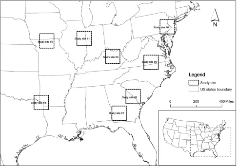
Eight study sites representing different landscape structure were chosen from the NLCD 2011 product. They are located in the central or eastern part of the United States. Each of them is a square region with a size of 180km×180km (Figure 1).
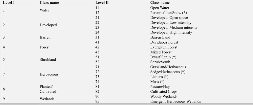
Two classification scheme levels were employed in this study (Table 1). Level II is the NLCD 2011 classification scheme with 15 classes common to all eight study sites. The scheme actually has other classes (e.g., Sedge/ Herbaceous in Alaska) which occur only in some regions of the US. Level I classes were generated by merging (collapsing) the thematic classes from level II into 8 classes. The preliminary analysis demonstrates that the cultivated/planted class dominates
study sites #1 and #2. Forest and cultivated/planted are the primary classes in study sites #3, #5, and #6. Developed, forest, and cultivated/planted are most prevalent in study site #4. Finally, study site #7 has a great quantity of cultivated/planted, forest, and wetland while forest, shrubland, cultivated/planted, and wetland are dominant in study site #8 (Table 2, Table 3).
Table 1. Two levels of legend and class scheme (The Level II is NLCD 2011 product legend and the classes names with (*) behind are not showed in the 8 study sites).
Level I Class name Level II Class name
1 Water 11 Open Water
12 Perennial Ice/Snow (*)
2 Developed
21 Developed, Open space
22 Developed, Low intensity
23 Developed, Medium intensity
24 Developed, High intensity
3 Barren 31 Barren Land
4 Forest
41 Deciduous Forest
42 Evergreen Forest
43 Mixed Forest
5 Shrubland 51 Dwarf Scrub (*)
52 Shrub/Scrub
7 Herbaceous
71 Grassland/Herbaceous
72 Sedge/Herbaceous (*)
73 Lichens (*)
74 Moss (*)
8 Planted/
Cultivated
81 Pasture/Hay
82 Cultivated Crops
9 Wetlands 90 Woody Wetlands
95 Emergent Herbaceous Wetlands
Table 2. Percentage of each thematic class for eight study sites using the first-level classification scheme (8 classes).
Level I Percentage of area (%)
Site 1 Site 2 Site 3 Site 4 Site 5 Site 6 Site 7 Site 8
1 0.61 1.05 0.80 2.37 2.80 1.82 0.62 2.07
2 8.04 5.04 7.62 29.01 5.98 7.43 5.94 7.78
3 0.06 0.05 0.42 0.52 0.29 0.19 0.14 0.45
4 7.74 18.79 55.22 33.02 45.37 56.77 36.85 37.27
5 0.02 0.87 0.69 2.43 8.09 5.33 4.03 10.71
7 0.67 2.17 4.31 0.48 5.21 5.86 6.44 8.07
8 82.39 70.01 30.90 23.28 23.48 19.88 32.13 15.84
9 0.47 2.03 0.04 8.89 8.78 2.72 13.83 17.81
Table 3. Percentage of each thematic class for eight study sites using the second-level classification scheme (15 classes).
Level II Percentage of area (%)
Site 1 Site 2 Site 3 Site 4 Site 5 Site 6 Site 7 Site 8
11 0.61 1.05 0.80 2.37 2.80 1.82 0.62 2.07
21 4.03 3.68 4.85 14.24 3.22 5.20 4.10 4.82
22 3.23 1.18 1.84 8.08 2.29 1.58 1.33 2.02
23 0.57 0.14 0.72 4.73 0.36 0.48 0.35 0.70
24 0.20 0.03 0.21 1.95 0.12 0.17 0.16 0.23
31 0.06 0.05 0.42 0.52 0.29 0.19 0.14 0.45
41 7.71 17.95 50.67 28.30 18.87 37.62 10.79 9.71
42 0.02 0.08 2.04 2.68 20.24 15.24 21.59 25.40
43 0.01 0.76 2.51 2.04 6.26 3.91 4.48 2.16
52 0.02 0.87 0.69 2.43 8.09 5.33 4.03 10.71
71 0.67 2.17 4.31 0.48 5.21 5.86 6.44 8.07
81 2.84 45.27 28.62 10.29 20.37 17.82 6.25 6.48
82 79.55 24.74 2.28 12.98 3.11 2.05 25.88 9.36
90 0.45 1.81 0.02 7.99 8.02 2.61 12.50 16.54
The landscape characteristics of the eight study sites were analyzed using the following indices: landscape shape index (LSI), mean patch size (Area_M), mean shape index (Shape_M), edge density (ED), and contagion index (CON) [24, 25]. LSI measures the overall geometric complexity of the entire landscape. Area_M evaluates the mean patch size while Shape_M assesses the complexity of patch shape compared to a square shape of the same size. ED denotes the length of edges per unit area. CON indicates both patch type interspersion and patch dispersion at the landscape level. This analysis was accomplished using Fragstats v4.2 designed for quantification and analysis of landscape metrics for categorical maps [26].
2.2. Data
2.2.1. Reference Data
The reference data for the eight study sites were obtained from the NLCD 2011 product [27]. Two levels of the classification scheme were generated for the reference data, and the spatial resolution is 30m (Table 1). We assumed that the thematic accuracy of the NLCD 2011 product is one hundred percent for purposes of this research so that the impact of positional error could be evaluated.
2.2.2. Soft Classification Data
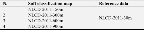
The soft classification maps of different spatial resolutions for each study site were generated by upscaling the reference data. Different window sizes, varying from 5×5 to 10×10, 20×20, and 30×30 pixels, were used to create the soft classification maps with spatial resolutions of 150, 300, 600, and 900 meters, respectively (Table 4). Each pixel in the soft classification map contains a vector denoting the proportion of each class. This upscaling method was applied to all reference data across each study site for both levels of the classification scheme.
There are several reasons that this research upscaled the reference data to generate soft classification maps instead of using other existing coarser land cover classification maps (e.g., land cover datasets classified from AVHRR or MODIS imagery). First, soft classification of coarser-resolution images introduces classification errors [28, 29], and various classification errors combined with varied positional errors would make the results difficult to explain. Second, it is nearly impossible to find such a series of soft classification maps for each study site with different spatial resolutions.
Table 4. Soft classification maps and their reference data.
N. Soft classification map Reference data
1 NLCD-2011-150m
NLCD-2011-30m
2 NLCD-2011-300m
3 NLCD-2011-600m
4 NLCD-2011-900m
2.3. Soft Classification Accuracy Assessment with Positional Errors
Suppose that a soft classification map has pixels and of them are randomly sampled for accuracy assessment. Soft
classification accuracy assessment with positional errors proceeds in the following way. The sampling pixel in the form of a vector v ( , ) at the location (x, y) in the soft
classification map takes the cluster of pixels at location (x + ∆, y + ∆) in the reference data as the validation unit which is in the form of a vector ( ∆, ∆). The error matrix
for the sampling pixel is then constructed using Eq. (1).
,∆= v ( , ) ∩ ( ∆, ∆) (1)
In Eq. (1), the construction rule ∩ is explained by a composite operator developed by Pontius and Cheuk [30] in which the diagonal and off-diagonal elements employ different algorithms. Generally, a minimum operator is calculated for the diagonal elements while the multiplication operator is carried out for the off-diagonal elements. The designing idea and details of calculation can be found in [30]. This composite operator has been widely accepted for its practical and simple characteristics [31]. # is the number of soft pixels shifted from its original position in the soft classification map and varied from 0 to 3 soft pixels with an addition of 0.1 soft pixels in order to measure the positional effect at sub-pixel level [32]. This translation model has been widely used to simulate positional errors [33, 34].
The final soft error matrix is created by averaging the soft error matrixes (Eq. (1)) for all sampling pixels ( ) [7, 8, 35]. Previous research has shown that sampling introduces errors affecting the accuracy measures [36]. Therefore, in this research all soft pixels in the classification map were included to avoid sampling errors.
This research was interested in the component of thematic error caused by positional errors. This part of the thematic error equals the absolute values of the accuracy measures without positional errors minus the counterpart with positional errors (Eq. (2, 3)). We calculated $%-' to indicate the part of thematic error for overall accuracy ($%),
and ( )) -' for ( )) . Although a few recent have
questioned the usefulness of kappa [37], kappa is still widely used in global land cover mapping such as [38-40]. Besides, the focus of this research is not on kappa itself, but rather the positional effect on ( )) . This analysis will promote additional and necessary attention on the impact that position has on soft classification accuracy assessment.
$%-' = |$%∆+,− $%∆.,| (2)
( )) -' = |( )) ∆+,− ( )) ∆.,| (3)
3. Results
3.1. Landscape Characteristics and the Mixed Pixels’ Percentage of the Eight Study Sites
to 123.65 meters/hectare, and from 77.59 to 40.71, respectively for the level I classification scheme. The indices of LSI, Area_M, and ED present a trend that landscape characteristics become more complex and heterogeneous from study site #1 to #8. This trend keeps approximately the
same for the level II classification scheme apart from study sites #7 and #8. Table 5 also shows the percentage of mixed pixels in these soft classification maps. Obviously, a bigger window size (lower spatial resolution), combined with more heterogeneous landscape, increases this percentage.
Table 5. Landscape characteristics and the mixed pixels’ percentage of the eight study sites for both level I and II classification schemes.
Sites LSI Area_m Shape_m ED CON 150m 300m 600m 900m
Level 1: (8 classes) Percentage of mixed pixels (%)
Site 1 210.30 60.06 1.81 46.51 77.59 33.73 54.57 79.42 92.01
Site 2 349.02 19.77 1.74 77.34 65.89 55.20 80.70 96.50 99.36
Site 3 382.43 19.23 1.89 84.76 61.22 56.90 78.99 94.01 98.13
Site 4 425.88 15.56 1.81 94.42 49.56 60.67 81.33 93.10 96.45
Site 5 487.70 13.53 1.94 108.15 46.81 65.33 86.20 96.95 99.04
Site 6 497.92 12.01 1.90 110.43 52.23 69.07 88.87 97.67 99.15
Site 7 515.37 9.78 1.87 114.30 47.00 70.07 90.81 98.80 99.77
Site 8 557.64 9.25 1.92 123.65 40.72 72.36 90.28 97.59 99.03
Level 2: (15 classes) Percentage of mixed pixels (%)
Site 1 250.66 24.29 1.96 55.56 77.63 36.72 57.29 81.07 92.87
Site 2 446.96 12.30 1.88 99.10 60.88 65.49 89.01 98.84 99.85
Site 3 493.54 9.96 1.88 109.45 60.80 65.80 85.36 96.51 99.08
Site 4 717.06 6.30 1.90 159.12 41.73 80.42 92.79 97.73 99.00
Site 5 721.54 6.05 1.97 160.12 41.53 80.22 94.36 98.83 99.48
Site 6 746.56 5.25 1.86 165.68 46.13 85.87 97.29 99.49 99.85
Site 7 717.38 4.83 1.86 159.20 42.49 80.52 95.33 99.61 99.93
Site 8 717.39 5.49 1.91 159.20 40.21 82.04 95.09 98.85 99.54
3.2. Impact of Positional Errors on OA and Kappa Derived from the Soft Error Matrix
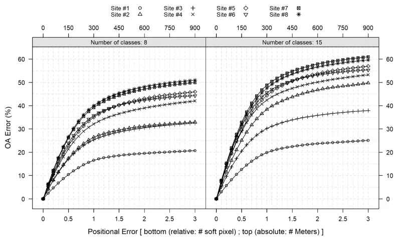
Figures 2-5 show the OA-errors when positional errors varied from 0.1 soft pixels to 3 pixels while Figures 6-9 present the Kappa-errors accordingly when the spatial resolution is 150, 300, 600, and 900 meters, respectively. Each figure is divided into two groups by the classification scheme (8 classes or 15 classes). Within each group, each type of line represents one study site with specific landscape characteristics. The bottom abscissa value ranging from 0 to 3 indicates the amount of the soft pixels associated with a given spatial resolution while the top value denotes the absolute distance in meters correspondingly.
Figure 2 demonstrates the impact of positional errors on overall accuracy of eight study sites at a spatial resolution of 150 meters. Within the group using the 8-class scheme, the rate of growth depends on the spatial characteristic of each study site. For example, the rate of growth of study site #1 is the lowest as a result of its most homogeneous landscape pattern with the simplest shapes and largest patch sizes. The rate of growth of study site #8 is the highest because it has the most heterogeneous landscape pattern with the most complex shapes and smallest patch sizes. The slope of each line is steeper at the beginning and then becomes more stable. The trend and shape of the lines between study site #2 and #3 are similar. The same situation also occurs between study site #5 and #6, and between study site #7 and #8. At the positional error of 0.5 pixels, the OA-error is 9.49% for study site #1 and increases to 24.28% for study site #8. Generally, the lines in the left group are lower than the corresponding ones in the right group, which indicates that a higher number of categorical classes increases the positional
effect. For instance, at the positional error of 3 soft pixels, the OA-error of study site #8 is 53.56% using the 8-class scheme while the OA-error is 62.94% for the 15-class scheme. It can also be seen that the order of lines in the right group changes such that the highest line is from study site #7.
The results found in Figure 3 are very similar to Figure 2 when the spatial resolution is 300 meters. The only difference is that the spatial resolution of 300 meters creates a less positional effect on OA-error than the spatial resolution of 150 meters does with the same amount of absolute distance. The same is true for relative distance. For example, the positional error of 300 meters creates 49.28% of OA-error at study site #8 when the spatial resolution is 150 meters in the 8-class scheme whereas the positional effect drops to 39.98% when the spatial resolution is 300 meters. Three soft pixels’ positional error creates 53.56% of OA-error at study site #8 when the spatial resolution is 150 meters while the value decreases to 50.97% at the spatial resolution of 300 meters.
The results in Figure 4 are different from what has been found in both Figures 2 and 3 when the spatial resolution becomes 600 meters. The line of study site #1 shows a trend becoming stable when the positional error reaches one soft pixel in the 8-class group as does the lines for study sites #2, #3, and #6. The lines of study site #1 and #3 show the same trend in the 15-class scheme. The relative comparison between the study sites stays the same except the line for study site #4 which is higher than the line of study site #6 when the positional errors exceeds1.9 and 1.7 soft pixels in the 8 and 15 class schemes, respectively.
respectively.
The comparison of Figure 2 to Figure 5, when holding the classification scheme constant, shows that the spatial resolution alters the impact of positional errors on the OA-error. For example, for study site #1, the OA-error varies from 0 to 20.19% at the spatial resolution of 150 meters in contrast to the variation from 0 to 17.93% at the spatial resolution of 900 meters.
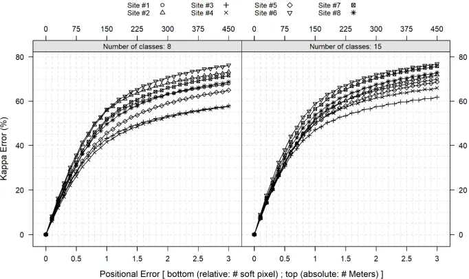
The analysis performed with OA-error is same for Kappa-error (Figures 6-9). Few differences exist between the results of OA-error and Kappa-error. First, compared to the positional effect on the overall accuracy, the impact on the kappa is higher. For example, with three soft pixels’
positional errors, the Kappa-error ranges from 0 to 76.83% while the OA-error varies from 0 to 64.1%. Second, the lines of study sites become much denser in contrast to the ones in the analysis of OA-error. Third, the lines in the 8 classes’ group are much lower than the corresponding lines in the 15 classes’ group however the degree is not as much as they are showed in the OA-error analysis. Fourth, the spatial resolution changes the lines’ pattern more than it does in the OA-error analysis. For example, in the 15 classes’ group, the highest line is the study site #6 at the spatial resolution of 150m, and it becomes the line of study site #1 at the spatial resolution of 900m.
Figure 2. Impact of positional errors on OA-error of eight study sites with two levels of classification scheme at the spatial resolution of 150 meters.
Figure 4. Impact of positional errors on OA-error of eight study sites with two levels of classification scheme at the spatial resolution of 600 meters.
Figure 5. Impact of positional errors on OA-error of eight study sites with two levels of classification scheme at the spatial resolution of 900 meters.
Figure 7. Impact of positional errors on Kappa-error of eight study sites with two levels of classification scheme at the spatial resolution of 300 meters.
Figure 8. Impact of positional errors on Kappa-error of eight study sites with two levels of classification scheme at the spatial resolution of 600 meters.
3.3. The Required Registration Accuracy for Soft Classification Accuracy Assessment
Table 6 shows the required registration accuracies (# of soft pixels) to keep both OA-error and Kappa-error under 10% for eight study sites with two levels of classification scheme at a spatial resolution of 150, 300, 600, and 900 meters, respectively. To retain OA-error less than 10% for the 8 classes’ scheme, the required registration accuracy for spatial resolution of 150, 300, 600, and 900meters ranges from 0.1 to 0.5 soft pixels, from 0.1 to 0.4 soft pixels, from
0.1 to 0.4 soft pixels, and from 0.1 to 0.5 soft pixels, respectively. It is clear that half of a soft pixel is not enough to obtain an OA-error of less than 10%. As the spatial resolution becomes coarser, the required registration accuracy decreases from 0.20 to 0.18 for the overall accuracy. The 15-class scheme makes achieving the required registration accuracy more difficult. To keep the Kappa-error lower than 10%, the required registration accuracy should reach 0.1 soft pixels for all spatial resolutions and both classification schemes.
Table 6. The required registration accuracy (# soft pixel) to keep the OA and Kappa error under 10% for eight study sites at the spatial resolutions of 150, 300, 600, and 900 meters, respectively. (< representing “less than”).
Sites Less than 10% OA-error Less than 10% Kappa-error
150 300 600 900 150 300 600 900
First level: 8 classes
Site #1 0.5 0.4 0.4 0.5 0.1 0.1 0.1 0.1
Site #2 0.2 0.2 0.2 0.2 0.1 0.1 0.1 0.1
Site #3 0.2 0.2 0.2 0.2 0.1 0.1 0.1 0.1
Site #4 0.2 0.2 0.2 0.2 0.1 0.1 0.1 0.1
Site #5 0.2 0.1 0.1 0.1 0.1 0.1 0.1 0.1
Site #6 0.1 0.1 0.1 0.1 0.1 0.1 0.1 0.1
Site #7 0.1 0.1 0.1 0.1 0.1 0.1 0.1 0.1
Site #8 0.1 0.1 0.1 0.1 0.1 0.1 0.1 0.1
Average 0.20 0.18 0.18 0.18 0.10 0.10 0.10 0.10
Second level: 15 classes
Site #1 0.4 0.3 0.3 0.3 0.1 0.1 0.1 0.1
Site #2 0.2 0.1 0.1 0.1 0.1 0.1 0.1 0.1
Site #3 0.2 0.2 0.2 0.2 0.1 0.1 0.1 0.1
Site #4 0.1 0.1 0.1 0.1 0.1 0.1 0.1 0.1
Site #5 0.1 0.1 0.1 0.1 0.1 0.1 0.1 0.1
Site #6 0.1 0.1 0.1 0.1 0.1 0.1 0.1 0.1
Site #7 0.1 0.1 0.1 0.1 0.1 0.1 0.1 0.1
Site #8 0.1 0.1 0.1 0.1 0.1 0.1 0.1 0.1
Average 0.16 0.14 0.14 0.14 0.10 0.10 0.10 0.10
4. Discussion
Soft classification methods have provided an impetus for transforming the hard classification error matrix into a soft one. However, the assumptions applied for the hard classification error matrix may not be suitable for the soft one. This research examined the impacts of positional errors on the thematic accuracy measures derived from the soft error matrix using NLCD 2011 as reference data and several coarser maps generated from NLCD 2011 as classification maps at the spatial resolutions of 150m, 300m, 600m, and 900m. Eight study sites, with a spatial extent of 180km × 180km, of different landscape characteristics were investigated using two levels of classification scheme. The thematic errors caused by positional errors were reported using OA-error and Kappa-error.
Our results are consistent with the results found in the simulation experiment [20] but have now been verified with actual, existing maps and not just simulations. For example, the positional effect becomes greater where the landscape is more heterogeneous. Also, the positional effect is reduced when the spatial resolution becomes coarser. The kappa
values were more sensitive to positional error than overall accuracy. As a result, the following analysis and discussion focus mainly on new findings that complement what has been found in the previous simulation experiments.
10%. Also, most of the global land cover datasets contain more than 15 classes. Therefore, we can speculate that the errors in the overall accuracy and kappa would be higher. This implication raises the issue of the reliability of thematic accuracies reported by these global mapping projects and highlights the importance of uncertainty analysis of thematic
accuracies based on positional errors. Such an analysis would improve the confidence level of further research based on these land cover datasets. This research strongly recommends the additional uncertainty analysis due to positional errors in future global land cover mapping.
Table 7. Thematic accuracy and positional accuracy of the selected global land cover database.
N. IGBP UMD MODIS 5 GLC 2000 GlobCover 2009
1 Input data AVHRR AVHRR MODIS SPOT-VEGETATION MERIS
2 Collection date 1992-1993 1992-1993 2001-2008 1999-2000 2009
3 N. of classes 17 14 5 different classification schemes 22 22
3 Spatial resolution 1km 1km 500m 1km 300m
4 Thematic accuracy 66.9% unknown 74.8% 68.6% 67.5%
5 Positional accuracy ~1km ~1km 50-100m 300m-333m 77m
6 Reference [10, 41] [12, 42] [43, 44] [5, 45] [6, 14]
Global land cover mapping made use of images at the spatial resolution of 1km such as MODIS and AVHRR [3, 4] and preferred finer images such as MERIS [6, 14]. Most of them were validated by Landsat images [21-23]. This paper determined that a half-pixel is not suitable for soft classification accuracy assessment at these scales using Landsat images as reference. To keep the thematic errors due to positional errors less than 10%, the required registration accuracy should achieve 0.14 pixels for overall accuracy and 0.10 pixels for kappa for the 8-class scheme. This requirement increases to 0.10 pixels for both overall accuracy and kappa for the 15-class scheme. As the spatial resolution becomes coarser, and the classification scheme includes more map classes, the positional requirement increases. Therefore, the positional accuracy standard for the soft classification accuracy assessment should be updated, and the future requirement for registration accuracy must consider the spatial resolution, number of classes in the classification scheme and the spatial characteristics of the imagery. Considering more land cover and land use maps were produced by soft classification [46-49] and given the positional accuracies existing global land cover maps achieved, there is a great need to improve image registration methods or develop methods to eliminate the positional effect on soft classification accuracy assessment. Several techniques have been suggested to remove the positional effect for hard classification accuracy assessment such as spatial aggregation (e.g. 3×3 pixels) [34, 50-53] and fuzzy location model [54, 55]. However, whether they are appropriate for soft classification accuracy assessment needs further research.
The results also showed that the effect of positional errors is higher in the 15-class scheme than in the 8-class scheme as indicated by both OA-error and kappa-error. This result is reasonable because the landscape characteristics with more classes become more complex (Table 5). Nevertheless, surprisingly this trend becomes weaker if using kappa-error is used as an indicator as shown in Figures 6 to 9. Besides, compared to the effect on overall accuracy the highest and lowest positional impact on kappa was not study site #8 and #1, respectively regardless of spatial resolution. Even worse
is that the highest positional impact on kappa is at study site #1 when the spatial resolution is 900m. The underlying reason for these unexpected results is that user accuracy or producer accuracy of classes with smaller proportions caused by positional error seems to approximate zero, which makes the kappa value quite low despite the relatively high value of overall accuracy. This also demonstrates that kappa is inconsistent with overall accuracy, which is proof to confirm that kappa does provide discrepant accuracy information.
5. Conclusions
of classes. There is a great need to update the positional requirements for soft accuracy assessment according to the image spatial resolution, classification scheme, and landscape structure. Besides, techniques suggested to remove positional effect in hard classification may not be appropriate for soft one, which needs to be investigated further. Considering positional issues and analysis described in this paper will significantly improve soft accuracy assessment in the future.
Acknowledgements
Partial funding was provided by the New Hampshire Agricultural Experiment Station. This is Scientific Contribution Number: 2834. This work was supported by the USDA National Institute of Food and Agriculture McIntire Stennis Project #NH00095 (Accession #1015520). The authors would like to thank the anonymous reviewers for their helpful suggestions and insightful comments that greatly improved our manuscript.
References
[1] Giri, C., et al., Next generation of global land cover characterization, mapping, and monitoring. International Journal of Applied Earth Observation and Geoinformation, 2013. 25 (1): p. 30-37.
[2] Sahle, M. and K. Yeshitela, Dynamics of land use land cover and their drivers study for management of ecosystems in the socio-ecological landscape of Gurage Mountains, Ethiopia. Remote Sensing Applications: Society and Environment, 2018. 12: p. 48-56.
[3] Wang, Y., et al., Remote sensing of land-cover change and landscape context of the National Parks: A case study of the Northeast Temperate Network. Remote Sensing of Environment, 2009. 113 (7): p. 1453-1461.
[4] Yin, H., et al., Mapping Annual Land Use and Land Cover Changes Using MODIS Time Series. Ieee Journal of Selected Topics in Applied Earth Observations and Remote Sensing, 2014. 7 (8): p. 3421-3427.
[5] Bartholomé, E. and A. Belward, GLC2000: a new approach to global land cover mapping from Earth observation data. International Journal of Remote Sensing, 2005. 26 (9): p. 1959-1977.
[6] Bontemps, S., et al., GlobCover 2009: products description and validation report. URL: http://ionia1. esrin.esa.int/docs/GLOBCOVER2009_Validation_Report _2, 2011. 2.
[7] Congalton, R. G., A review of assessing the accuracy of classifications of remotely sensed data. Remote Sensing of Environment, 1991. 37 (1): p. 35-46.
[8] Congalton, R. G. and K. Green, Assessing the accuracy of remotely sensed data: principles and practices. 2019: CRC press.
[9] Story, M. and R. G. Congalton, ACCURACY ASSESSMENT - A USERS PERSPECTIVE. Photogrammetric Engineering and Remote Sensing, 1986. 52 (3): p. 397-399.
[10] Husak, G. J., B. C. Hadley, and K. C. McGwire, Landsat thematic mapper registration accuracy and its effects on the IGBP validation. Photogrammetric Engineering and Remote Sensing, 1999. 65 (9): p. 1033-1039.
[11] Hansen, M. C. and B. Reed, A comparison of the IGBP DISCover and University of Maryland 1 km global land cover products. International Journal of Remote Sensing, 2000. 21 (6-7): p. 1365-1373.
[12] McCallum, I., et al., A spatial comparison of four satellite derived 1 km global land cover datasets. International Journal of Applied Earth Observation and Geoinformation, 2006. 8 (4): p. 246-255.
[13] Friedl, M. A., et al., Global land cover mapping from MODIS: algorithms and early results. Remote Sensing of Environment, 2002. 83 (1–2): p. 287-302.
[14] Defourny, P., et al. Accuracy assessment of global land cover maps: lessons learnt from the GlobCover and GlobCorine experiences. in 2010 European Space Agency Living Planet Symposium. 2010.
[15] Powell, R. L., et al., Sources of error in accuracy assessment of thematic land-cover maps in the Brazilian Amazon. Remote Sensing Of Environment, 2004. 90 (2): p. 221-234.
[16] Brown, K. M., G. M. Foody, and P. M. Atkinson, Modelling geometric and misregistration error in airborne sensor data to enhance change detection. International Journal of Remote Sensing, 2007. 28 (12): p. 2857-2879.
[17] Eastman, R. D., et al., Research issues in image registration for remote sensing, in 2007 Ieee Conference on Computer Vision and Pattern Recognition, Vols 1-8. 2007. p. 3233-3240. [18] Verbyla, D. L. and T. O. Hammond, Conservative bias in classification accuracy assessment due to pixel-by-pixel comparison of classified images with reference grids. International Journal of Remote Sensing, 1995. 16 (3): p. 581-587.
[19] Stehman, S. V. and J. D. Wickham, Pixels, blocks of pixels, and polygons: Choosing a spatial unit for thematic accuracy assessment. Remote Sensing of Environment, 2011. 115 (12): p. 3044-3055.
[20] Gu, J. Y., R. G. Congalton, and Y. Z. Pan, The Impact of Positional Errors on Soft Classification Accuracy Assessment: A Simulation Analysis. Remote Sensing, 2015. 7 (1): p. 579-599.
[21] Mayaux, P., et al., Validation of the global land cover 2000 map. Ieee Transactions on Geoscience and Remote Sensing, 2006. 44 (7): p. 1728-1739.
[22] Scepan, J., Thematic validation of high-resolution global land-cover data sets. Photogrammetric Engineering and Remote Sensing, 1999. 65 (9): p. 1051-1060.
[23] Zhao, Y. Y., et al., Towards a common validation sample set for global land-cover mapping. International Journal of Remote Sensing, 2014. 35 (13): p. 4795-4814.
[24] Uuemaa, E., et al., Landscape metrics and indices: an overview of their use in landscape research. Living reviews in landscape research, 2009. 3 (1): p. 1-28.
[26] McGarigal, K. and B. J. Marks, FRAGSTATS: spatial pattern analysis program for quantifying landscape structure. Gen. Tech. Rep. PNW-GTR-351. Portland, OR: US Department of Agriculture, Forest Service, Pacific Northwest Research Station. 122 p, 1995. 351.
[27] Wickham, J., et al., Thematic accuracy assessment of the 2011 National Land Cover Database (NLCD). Remote Sensing of Environment, 2017. 191: p. 328-341.
[28] Doan, H. T. X. and G. M. Foody, Increasing soft classification accuracy through the use of an ensemble of classifiers. International Journal of Remote Sensing, 2007. 28 (20): p. 4609-4623.
[29] Mackin, K. J., et al., Land Surface Cover Classification by Soft Computing Methods using MODIS Satellite Data. Information-an International Interdisciplinary Journal, 2010. 13 (3B): p. 1013-1018.
[30] Pontius, R. G. and M. L. Cheuk, A generalized cross-tabulation matrix to compare soft-classified maps at multiple resolutions. International Journal of Geographical Information Science, 2006. 20 (1): p. 1-30.
[31] Patidar, N. and A. K. Keshari, A multi-model ensemble approach for quantifying sub-pixel land cover fractions in the urban environments. International Journal of Remote Sensing, 2018. 39 (12): p. 3939-3962.
[32] Van Niel, T. G., et al., The impact of misregistration on SRTM and DEM image differences. Remote Sensing of Environment, 2008. 112 (5): p. 2430-2442.
[33] Dai, X. L. and S. Khorram, The effects of image misregistration on the accuracy of remotely sensed change detection. Ieee Transactions on Geoscience and Remote Sensing, 1998. 36 (5): p. 1566-1577.
[34] Chen, G., K. Zhao, and R. Powers, Assessment of the image misregistration effects on object-based change detection. ISPRS Journal of Photogrammetry and Remote Sensing, 2014. 87 (0): p. 19-27.
[35] Foody, G. M., Sample size determination for image classification accuracy assessment and comparison. International Journal of Remote Sensing, 2009. 30 (20): p. 5273-5291.
[36] Plourde, L. and R. G. Congalton, Sampling method and sample placement: How do they affect the accuracy of remotely sensed maps? Photogrammetric Engineering and Remote Sensing, 2003. 69 (3): p. 289-297.
[37] Pontius, R. G., Jr. and M. Millones, Death to Kappa: birth of quantity disagreement and allocation disagreement for accuracy assessment. International Journal of Remote Sensing, 2011. 32 (15): p. 4407-4429.
[38] Chen, J., et al., Global land cover mapping at 30m resolution: A POK-based operational approach. ISPRS Journal of Photogrammetry and Remote Sensing, 2015. 103: p. 7-27. [39] Liu, X., et al., High-resolution multi-temporal mapping of
global urban land using Landsat images based on the Google Earth Engine Platform. Remote Sensing of Environment, 2018. 209: p. 227-239.
[40] Wang, J., et al., Mapping global land cover in 2001 and 2010
with spatial-temporal consistency at 250m resolution. ISPRS Journal of Photogrammetry and Remote Sensing, 2015. 103: p. 38-47.
[41] Loveland, T., et al., Development of a global land cover characteristics database and IGBP DISCover from 1 km AVHRR data. International Journal of Remote Sensing, 2000. 21 (6-7): p. 1303-1330.
[42] Hansen, M. C., et al., Global land cover classification at 1 km spatial resolution using a classification tree approach. International Journal of Remote Sensing, 2000. 21 (6-7): p. 1331-1364.
[43] Mora, B., et al., Global land cover mapping: Current status and future trends, in Land Use and Land Cover Mapping in Europe. 2014, Springer. p. 11-30.
[44] Friedl, M. A., et al., MODIS Collection 5 global land cover: Algorithm refinements and characterization of new datasets. Remote Sensing of Environment, 2010. 114 (1): p. 168-182. [45] Mayaux, P., et al., A new land-cover map of Africa for the
year 2000. Journal of Biogeography, 2004. 31 (6): p. 861-877. [46] Zhang, B., et al., Land use and land cover classification for
rural residential areas in China using soft-probability cascading of multifeatures. Journal of Applied Remote Sensing, 2017. 11: P. 1-17.
[47] Chen, Y. H., et al., Subpixel Land Cover Mapping Using Multiscale Spatial Dependence. Ieee Transactions on Geoscience and Remote Sensing, 2018. 56 (9): p. 5097-5106. [48] Ma, A. L., et al., Multiobjective Subpixel Land-Cover
Mapping. Ieee Transactions on Geoscience and Remote Sensing, 2018. 56 (1): p. 422-435.
[49] Suresh, M. and K. Jain, Subpixel level mapping of remotely sensed image using colorimetry. Egyptian Journal of Remote Sensing and Space Sciences, 2018. 21 (1): p. 65-72.
[50] Carmel, Y., Controlling Data Uncertainty via Aggregation in Remotely Sensed Data. Ieee Geoscience And Remote Sensing Letters, 2004. 1 (2): p. 39-41.
[51] Zhang, M., et al., Impacts of Plot Location Errors on Accuracy of Mapping and Scaling Up Aboveground Forest Carbon Using Sample Plot and Landsat TM Data. IEEE GEOSCIENCE AND REMOTE SENSING LETTERS, 2013. 10 (6): p. 1483.
[52] Tan, B., et al., The impact of gridding artifacts on the local spatial properties of MODIS data: Implications for validation, compositing, and band-to-band registration across resolutions. Remote Sensing of Environment, 2006. 105 (2): p. 98-114. [53] Congalton, R. G. Thematic and positional accuracy
assessment of digital remotely sensed data. in Proceedings of the 7th annual forest inventory and analysis symposium. 2005. [54] Huang, Z. and B. G. Lees, Assessing a single classification accuracy measure to deal with the imprecision of location and class: Fuzzy weighted Kappa versus Kappa. Journal of Spatial Science, 2007. 52 (1): p. 1-12.