Computer-Aided, Multi-Modal, and Compression Diffuse Optical Studies of Breast Tissue

(1)

University of Pennsylvania

ScholarlyCommons

Publicly Accessible Penn Dissertations

Fall 12-22-2011

Computer-Aided, Multi-Modal, and Compression

Diffuse Optical Studies of Breast Tissue

David R. Busch Jr

University of Pennsylvania, [email protected]

Follow this and additional works at:

http://repository.upenn.edu/edissertations

Part of the

Bioimaging and Biomedical Optics Commons,

Biological Engineering Commons,

Optics Commons, and the

Radiology Commons

This paper is posted at ScholarlyCommons.http://repository.upenn.edu/edissertations/438

For more information, please [email protected].

Recommended Citation

Busch, David R. Jr, "Computer-Aided, Multi-Modal, and Compression Diffuse Optical Studies of Breast Tissue" (2011).Publicly Accessible Penn Dissertations. 438.

(2)

Computer-Aided, Multi-Modal, and Compression Diffuse Optical Studies

of Breast Tissue

Abstract

Diffuse Optical Tomography and Spectroscopy permit measurement of important physiological parameters

non-invasively through ~10 cm of tissue. I have applied these techniques in measurements of human breast

and breast cancer. My thesis integrates three loosely connected themes in this context: multi-modal breast

cancer imaging, automated data analysis of breast cancer images, and microvascular hemodynamics of breast

under compression. As per the first theme, I describe construction, testing, and the initial clinical usage of two

generations of imaging systems for simultaneous diffuse optical and magnetic resonance imaging. The second

project develops a statistical analysis of optical breast data from many spatial locations in a population of

cancers to derive a novel optical signature of malignancy; I then apply this data-derived signature for

localization of cancer in additional subjects. Finally, I construct and deploy diffuse optical instrumentation to

measure blood content and blood flow during breast compression; besides optics, this research has

implications for any method employing breast compression, e.g., mammography.

Degree Type

Dissertation

Degree Name

Doctor of Philosophy (PhD)

Graduate Group

Physics & Astronomy

First Advisor

Arjun G. Yodh

Keywords

diffuse optics, DOT, MRI, CAD, multi-modal imaging, compression, blood flow

Subject Categories

(3)

COMPUTER-AIDED, MULTI-MODAL, AND

COMPRESSION DIFFUSE OPTICAL STUDIES OF

BREAST TISSUE

David Richard Busch Jr.

A Dissertation

in

Physics and Astronomy

Presented to the Faculties of the University of Pennsylvania in Partial

Fulfillment of the Requirements for the Degree of Doctor of Philosophy

2011

Supervisor of Dissertation

Arjun G. Yodh

James M. Skinner Professor of Science, Department of Physics and Astronomy

Graduate Group Chairperson

Alan T. Johnson

Professor, Department of Physics and Astronomy

Dissertation Committee

Mark Goulian, Associate Professor, Department of Physics and Astronomy

Edmund J. and Louise W. Kahn Endowed Term Associate Professor of Biology

Philip Nelson, Professor, Department of Physics and Astronomy

Burt A. Ovrut, Professor, Department of Physics and Astronomy

(4)

c

Copyright 2011

(5)

Acknowledgements

The simultaneous optical and MR breast imaging project discussed in Chapter 4-6 were the results

of a long standing collaboration between Prof. Arjun Yodh and Prof. Britton Chance. The late Prof.

Chance, in whose lab I was based for several years, consistently provided unique and simplified solutions

to scientific problem, often tying in a wide range of historical precedents. Dr. Xavier Intes and Jiangsheng

Yu constructed opto-electronics of the second generation (GenII, Chapter4-5) University of Pennsylvania

Optical/MR Imaging system used in much of my work; Dr. Intes also patiently taught me the concepts and

realities of time-domain instrumentation and analysis. Dr. Thomas Connick designed and constructed the

(GenII and GenIII Chapter4-6) electronics for MR Imaging. I thank Jun Zhang and Zhongyao Zhao, who

assisted in the GenII and GenIIm optical/MR clinical data collection, along with the research MR technical

team, Tanya Kurtz, and Doris Cain. Norman Butler patiently taught me how to run the MR scanners and

answered a huge number of naive questions on clinical procedures. Dr. Saurav Pathak spent a great deal

of time and effort in adapting and improving reconstruction software for diffuse optical tomography with

the GenIII optical-MR imaging system; the reconstructions in Chapter 6 are due to his work. Design,

construction, modification, and repair of theses multi-modal instruments were heavily dependent on the

skills of the instrumentation specialists in the Department of Physics and School of Medicine, especially

Mike Carman, William Pennie, and Harold (‘Buddy’) Borders. Barry Chen, David L. Minkoff, and Daniel

Friedman assisted in various opto-electronic instrumentation used in the work described in Chapter4-6; Han

Y. Ban’s assistance in construction and debugging were especially helpful.

Moving novel instrumentation into clinical settings is fraught with difficulty; Dr. Mark A. Rosen and

Dr. Mitchell D. Schnall were instrumental in providing the opportunity to apply our instrumentation during

their clinical research MRI studies. They also greatly assisted in clinical data collection and introduced me

to clinical breast imaging. The ABI clinical coordinator team of Kathleen Thomas, Tamara April, Deborah

Arnold, and Stephanie Damia, was extremely helpful in recruiting subjects for our study.

Dr. Mary Putt and Dr. Wensheng Guo provided guidance among statistical pitfalls as I put together the

work in Chapter7; Dr. Regine Choe was unstinting generous in her assistance, interpretation, and data sets.

Data used in this chapter was derived from work by Dr. Joseph P. Culver, Dr. Soren D. Konecky, Dr. Alper

Corlu, Dr. Kijoon Lee, Dr. Turgut Durduran, Dr. Regine Choe, Han Y. Ban, and Dr. Saurav Pathak. Our

clinical collaborators include Dr. Mark A. Rosen, Dr. Mitchell D. Schnall, Dr. Brian J. Czerniecki, Dr. Julia

Tchou, Dr. Douglas L. Fraker, and Dr. Angela DeMichele.

The compression study in Chapter 8 grew out of a series of conversations I had with Dr. Mark A.

Rosen; Dr. Turgut Durduran and Dr. Regine Choe helped guide it to practical application. Alpha Kamara,

(6)

opto-electronics; Jiaming Liang and Dr. Turgut Durduran in writing software; and Wesley Baker and Dr.

Turgut Durduran in data analysis. Dr. Daniel Chen significantly eased my interpretation of the response of

breast tissue to external loading. Our clinical coordinators Dalton Hance, Tiffany Alverna, Monika Koptyra,

and Ellen Foster made human testing possible.

I thank the other members of Dr. Yodh’s lab during my time at University of Pennsylvania not directly

involved in the projects above, especially Dr. Rickson C. Mesquita, Dr. Ulas Sunar, Dr. Soren D. Konecky,

Dr. Jonathan Fisher, and Aninidita Basu. Dr. Erin M. Buckley is a generous and helpful colleague, in whose

company I deciphered University of Pennsylvania’s regulations on graduation. My classmates at University

of Pennsylvania, especially Dr. Daniel Swetz, Dr. Charles Ratliff, Dr. Jesse Kinder, and Dr. Michelle Caler,

were of indubitable help in my graduate school career. Dr. Gregory Faris and Dr. George Alexandrakis

introduced me to diffuse optical theory and experiment.

Dr. Turgut Durduran and Dr. Regine Choe became my mentors during the second half of my PhD work;

their patience, insightful comments, and support were essential to its completion.

My parents, aunts, uncles, and, especially, siblings and cousins have supported, encouraged, and prompted

me throughout my education, as well as being a reservoir of esoteric facts and contacts; I particularly thank

Andrew, Megan, and Shannon. My first introduction to working science came from my uncle and godfather,

the late Prof. James J. O’Leary M.D., Ph.D., who introduced me to scientific inquiry, chess, and the use of

lasers to answer biological questions.

The clarity, readability, and science of Prof. Yodh’s papers drew me into University of Pennsylvania and

his lab. Prof. Yodh’s weekly lab meetings focused not only on extracting the important kernels amidst the

chaff of complicated data sets, but also on how to efficiently communicate results. His high standards and

patience defined my graduate career.

(7)

ABSTRACT

Computer-Aided, Multi-Modal, and Compression Diffuse Optical Studies

of Breast Tissue

David Richard Busch Jr.

Arjun G. Yodh

Diffuse Optical Tomography and Spectroscopy permit measurement of important physiological

param-eters non-invasively through_∼10 cm of tissue. I have applied these techniques in measurements of human

breast and breast cancer. My thesis integrates three loosely connected themes in this context: multi-modal

breast cancer imaging, automated data analysis of breast cancer images, and microvascular hemodynamics

of breast under compression.

As per the first theme, I describe construction, testing, and the initial clinical usage of two generations

of imaging systems for simultaneous diffuse optical and magnetic resonance imaging. The second project

develops a statistical analysis of optical breast data from many spatial locations in a population of cancers

to derive a novel optical signature of malignancy; I then apply this data-derived signature for localization

of cancer in additional subjects. Finally, I construct and deploy diffuse optical instrumentation to measure

blood content and blood flow during breast compression; besides optics, this research has implications for

(8)

List of Tables

2.1 Approximate Optical Properties in theNIRfor various tissues near 800nm. . . 5

2.2 Important quantities and symbols in diffuse optics. . . 6

2.3 Notation used in describing semi-infinite and slab solutions to the diffusion equation in both time and frequency domain. . . 10

2.4 Diffuse optical data types. . . 35

2.5 Notation for DOT reconstruction. . . 44

3.1 Summary of optically detectable physiological contrasts in breast cancer. . . 54

3.2 Summary of Clinical Optical-MRI systems for breast cancer. . . 63

4.1 Summary of Optical-MR imaging systems at Penn. . . 67

4.2 Information content of Optical and MRI measurements of breast cancer. . . 69

4.3 GenII/GenIIm Instrument Components . . . 71

5.1 Summery of subjects studied with the GenII and GenIIm with combined DOT and MR Imaging. . . 79

5.2 Bulk TD-DOS optical properties. . . 82

5.3 Correlations between regional DOS and MR parameters from 19 subjects using the GenII and GenIIm systems. . . 82

5.4 Parameters in Equation5.1. . . 85

5.5 Parameters in Equation5.2. . . 85

5.6 Correlations between regional DOS and MR parameters from 8 subjects using the GenII and GenIIm systems. . . 86

7.1 Demographic breakdown of cancers in CAD study. . . 129

7.2 Demographic breakdown of cancers in CAD study of benign lesions. . . 145

7.3 Comparison of change in tumor volume during chemotherapy, determined by DOT-CAD and clinical imaging modalities. . . 153

8.1 Existing work on pressure perturbation of optical signals in the breast. . . 162

(14)

8.3 Demographic data for 15 subjects in Version 2 compression study. . . 172

8.4 Demographic data for 5 subjects in Version 3 compression study, as described in Section

8.4.3. . . 177

8.5 Tabulation of Young’s Moduli of Breast Tissue, from the literature. . . 186

8.6 Non-linear stress-strain models of breast tissue, compared to results from Version 3

com-pression study. . . 186

C.1 Scattering agents used in DOS/DOT phantoms. . . 203

(15)

List of Figures

2.1 Images of light propagation through scattering media. . . 4

2.2 Schematic of light scattering in tissue. Most individual scattering events (black) are strongly forward biased with scattering path lengthls ∼10µm. However, many (∼100) of these forward scattering events can be lumped together into a single, isotropic, event (red) with reduced scattering path lengthl0 s∼1mm (blue). The absorption path length (not shown) in the diffusion regime is many timesl0 s. . . 5

2.3 Schematic of reflection of radiance off tissue-air boundary. . . 10

2.4 Schematic of geometry for extrapolated boundary condition between air and tissue. . . 13

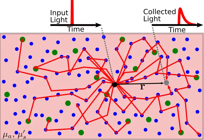
2.5 A schematic of a time domain measurement in an infinite homogeneous medium. . . 14

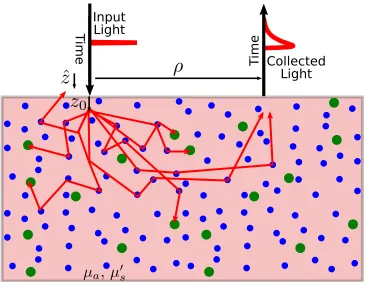
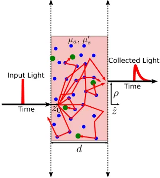
2.6 Schematic of semi-infinite (remission) geometry DOS, for a measurement on the input plane. 16 2.7 Schematic of infinite slab geometry DOS. . . 17

2.8 Notation for solutions to the photon diffusion equation in compressed breast (‘slab’) ge-ometry. . . 18

2.9 Graphs of Equation2.50for a slab varyingµa. . . 19

2.10 Graphs of Equation2.50for a slab varyingµ0 s. . . 20

2.11 Graphs of Equation2.50for a slab varyingρ. . . 21

2.12 Graphs of Equation2.56for a slab with varyingρ. . . 23

2.13 Conceptual Diffuse Correlation Spectroscopy (DCS) schematic. . . 25

2.14 Example of regularization parameter selection using an ‘L-Curve’. . . 32

2.15 A schematic of clinical coordinate system terminology. . . 38

2.16 Example of IRF, fitted theoretical curve, and data from a human subject. . . 40

2.17 An example of the effect of increasing absorption on TD data histograms. . . 40

2.18 Conceptual schematic of TD-DOS measurements. . . 41

3.1 Spectra of major breast tissue chromophores showing visible and NIR windows. . . 48

3.2 A schematic of a simple application of the Beer-Lambert Law. . . 48

(16)

3.4 DOT reconstructions of a 2.2 cm invasive ductal carcinoma. . . 52

3.5 DOT reconstructions of a 0.5 cm fibroadenoma. . . 53

3.6 Cartoon of tissue level organization of healthy and cancerous tissues. . . 54

3.7 Example blood flow contrast in cancerous and healthy breast tissue. . . 54

3.8 Results from optical-only kinetics imaging system. . . 57

3.9 ICG fluorescence contrast in 3D tomographic imaging of the human breast. . . 58

3.10 Test of influence of ICG on MRI signal from MultiHance (Gd chelate). . . 58

3.11 Example clinical work flow for breast cancer screening. . . 60

3.12 Cartoon of instrument and subject placement for simultaneous DOT and MRI measure-ment. . . 61

3.13 Simultaneous Optical and MRI measurements of ductal carcinoma by Ntziachristos, show-ing ICG and Gd-DTPA spatial correlation. . . 62

3.14 Information content of diffuse optical techniques. . . 64

4.1 Images and schematic of GenII Optical-MR Imaging system. . . 69

4.2 Opto-electronic schematic for GenII system. . . 71

4.3 Example TD-DOS data, collected with the GenII system. . . 72

4.4 Images of the GenII and GenIIm optical-MRI breast platform. . . 73

4.5 Optical/MRI Breast Imaging Platform schematic and images. . . 74

4.6 Schematic of the GenIIm system. . . 76

4.7 Kinetics phantom imaging with the GenIIm system. . . 77

5.1 Experimental time-line for (left) GenII and (right) GenIIm simultaneous clinical opti-cal/MRI measurements. . . 79

5.2 Example TD-DOS measurement of bulk optical properties of breast tissue with the GenII system. . . 81

5.3 Histograms of Hbtand StO2 measured with TD-DOS for all source-detector pairs in 19 subjects. . . 82

5.4 Example ICG uptake kinetics, measured with GenII and GenIIm systems. . . 83

5.5 Example ICG uptake curves on a single subject. . . 84

5.6 Example kinetics model fit to fractional changes in local MR image intensity due to Gd-DTPA uptake. The low temporal resolution of this data limits the complexity of kinetics models which may be applied. Note, the MR signal intensity is non-linearly related to the Gd-DTPA concentration. Data are solid blue circles. . . 85

5.7 Gd and mock ICG Contrast Enhanced Imaging; no clinical findings. . . 89

(17)

5.9 Example of Gd kinetics imaging in healthy tissue. . . 91

5.10 ICG and Gd Contrast Enhanced Imaging; invasive carcinoma outside of optical field of view. 92 5.11 Example of ICG kinetics imaging of healthy tissue. . . 93

5.12 Example of Gd kinetics imaging in healthy tissue. . . 94

5.13 ICG and Gd Contrast Enhanced Imaging; invasive carcinoma in optical field of view. . . . 95

5.14 Example of ICG kinetics imaging of an invasive ductal carcinoma. . . 96

5.15 Example of Gd kinetics imaging of an invasive ductal carcinoma. . . 97

5.16 Example segmentation of breast tissue into fat and glandular regions in a cancer-free breast. 98 5.17 Segmentation of Adipose and Tumor tissue using MRI data. . . 99

5.18 Comparison of ICG and Gd-DTPA kinetics, using tissue segmentation (Figure5.17) as a hard spatial prior. . . 100

5.19 Schematic and axial T1image showing fiber optic coupling of the GenIIm Opt-MR platform.101 5.20 Example of application of tissue shaping inserts in a single subject, tested with the GenIIm platform. . . 102

5.21 Example of difficulties with fiber optic placement in the GenII and GenIIm systems. . . 102

6.1 Photos of GenIII Optical-MR Imaging platform. . . 106

6.2 Several views of the GenIII Optical-MR Imaging platform. . . 106

6.3 Images of the lateral compression plates in the GenIII system. . . 107

6.4 A schematic of the compression plates for the GenIII system. . . 108

6.5 Photos of the GenIII Opt/MR platform during a phantom imaging study. . . 108

6.6 Example MR Imaging with GenIII platform. . . 109

6.7 Example detector fiber module for the GenIII system. . . 109

6.8 Example of GenIII source fiber module. . . 110

6.9 GenIII source and detector fiber modules. . . 110

6.10 GenIII detector modules and compression plates. . . 111

6.11 Schematic of GenIII current optical-MRI system. . . 112

6.12 Schematic of GenIII complete optical-MRI system. . . 113

6.13 CW detector optics for GenIII system. . . 113

6.14 Photos of the mobile opto-electronics system for GenIII. . . 114

6.15 GenIII phantom imaging: Slices through the target center in a 3D reconstruction of a multi-modality phantom from MR and DOT imaging. . . 116

6.16 Example phantom reconstructions from the GenIII system. . . 117

6.17 Initial human subject MR imaging with GenIII Opt/MR imaging platform. . . 118

(18)

7.1 Slices from 3D tomograms from subjects with breast cancer and optical property

distribu-tions for cancerous and healthy tissue. . . 126

7.2 Intra-subject data normalization brings inter-subject data distributions close to a normal distribution. . . 129

7.3 Example of masks applied to segment breast tissue for CAD. . . 130

7.4 Flow chart of CAD data processing for a single training subject. . . 131

7.5 Flow chart of CAD data analysis scheme. . . 133

7.6 Example of training and test set Malignancy Parameter and Probability of Malignancy. . . 136

7.7 An example of distributions of tissue optical properties. . . 137

7.8 Two examples of distributions of tissue optical properties. . . 137

7.9 Example Probability of Malignancy calculated for two test subjects. . . 138

7.10 Slices from 3D images of subjects in Figure7.9, showing total hemoglobin concentration, Probability of Malignancy, and a binary cancer mask. . . 140

7.11 Malignancy Parameter and Probability of Malignancy for the healthy and tumor regions of 35 test subjects. . . 141

7.12 Box plot of calculated probability of malignancy for each tumor voxel in all 35 malignant cancers, separated by diagnosis. . . 142

7.13 ROC curve and Classification Rates for each of 35 test subjects. . . 143

7.14 Comparison of voxel calculated probability of malignancy for cancerous, benign, and healthy regions. . . 145

7.15 Regionally averaged comparison of probability of malignancy between cancerous, benign, and healthy regions. . . 146

7.16 Distribution of probability of malignancy by type of benign lesion. . . 147

7.17 Examples of a three level mask of Probability of Malignancy segmenting healthy, suspi-cious, and malignant regions. . . 147

7.18 Intra-subject data normalization brings inter-subject data distributions close to a normal distribution. . . 148

7.19 Malignancy Parameter and Probability of Malignancy for each of 35 test subjects used in the CAD study. . . 149

7.20 Probability of Malignancy calculated for for each tumor voxel in 35 malignant cancers, separated by diagnosis. . . 149

7.21 Distribution of probability of malignancy by type of benign lesion. . . 150

(19)

7.23 ROC curve and Classification Rates for each of 35 test subjects with Hb, HbO2, andµ0

s. . . 151

7.24 Slices of 3D Probability of Malignancy map at 4 time points during chemotherapy treatment.153 7.25 Change in volume of high Probability of Malignancy during chemotherapy treatment, cal-culated from DOT-CAD. . . 153

8.1 Cartoon of blood vessel growth in cancer compared with the normal hierarchical structure of blood vessels in healthy tissue. . . 159

8.2 Schematic and photograph of modular DCS system. . . 164

8.3 Schematic and photograph of Version 1 compression system. . . 165

8.4 Time-line for compression study, Version 1. . . 166

8.5 TD measurements of chromophore changes during compression of human breast tissue. . . 167

8.6 Relative Blood Flow measurements in a 1 subject pilot study of transverse TD-DOS and DCS in the human breast. . . 168

8.7 Time line for Version II instrumentation for continuous measurement of optical properties during mammographic compression. . . 169

8.8 Example data from a single subject during breast compression. . . 170

8.9 Example data from breast tissue in six subjects during mammogram-like compression. . . 171

8.10 Change in measured pressure during compression at consistent distance with Version 2 system. . . 172

8.11 Scatter plot of changes in Hbt, StO2, and rBF in breast during compression from the Version 2 system. . . 173

8.12 Design for multi-sensitivity, multi-position pressure mapping compression plate with 2 source and 2 detector positions. . . 175

8.13 Updated compression plate system for optical measurements during mammographic com-pression. . . 176

8.14 Schematic of the experimental time-line for the Version 3 mammographic compression study. . . 176

8.15 Load, Plate Separation, Pressure,µ0 s, Hbt, StO2, and rBF during breast compression on a healthy volunteer. . . 178

8.16 Load, Plate Separation, Pressure,µ0 s, Hbt, StO2, and rBF during breast compression on a healthy volunteer. . . 179

8.17 Observed changes in blood oxygenation (StO2) versus Load, Pressure, and change in plate separation using the Version 3 compression system. . . 181

(20)

8.19 Observed changes in relative blood flow (rBF) versus Load, Pressure, and change in plate

separation using the Version 3 compression system. . . 183

8.20 Comparison between Load, Pressure, and change in plate separation using the Version 3

compression system. . . 185

8.21 Comparison of applied Load and Pressure to fractional change in plate separation (strain)

using the Version 3 compression system. . . 187

8.22 Portable TD and DCS system. . . 189

A.1 Schematic of two-compartment model from Cuccia. . . 193

B.1 Observed changes in blood oxygenation (StO2) versus Load, Pressure, and change in plate

separation using the Version 3 compression system, with confidence intervals. . . 196

B.2 Observed changes in total hemoglobin concentration (Hbt) versus Load, Pressure, and

change in plate separation using the Version 3 compression system. . . 197

B.3 Observed changes in relative blood flow (rBF) versus Load, Pressure, and change in plate

separation using the Version 3 compression system. . . 198

B.4 Comparison between Load, Pressure, and change in plate separation using the Version 3

compression system. . . 199

B.5 Comparison of applied Load and Pressure to fractional change in plate separation (strain)

using the Version 3 compression system. . . 200

(21)

Chapter 1 Introduction and Organization

Diffuse Optical Spectroscopy (DOS) utilizes light in the low absorption near-infra red (NIR) window,

be-tween 650 and 950 nm, to measure chromophore concentrations and scattering in thick tissues, e.g., through

∼10 cm of human breast tissue. Information about tissue concentrations of water, lipid, oxy- (HbO2), deoxy-(Hb), and total-hemoglobin (Hbt), as well as blood oxygen saturation (StO2), and tissue scattering (i.e., the reduced scattering coefficient, µ0

s) are readily derived using diffuse optics. These non-invasive, low-risk

diagnostics are emerging as useful clinical tools for detection, diagnosis, and monitoring of breast cancer1

and other pathologies2–4_{. Indeed, various studies have successfully compared Diffuse Optical Tomography}

(DOT) and DOS against more established clinical modalities5–11 _{and have correlated pathologic findings}

with optically measured chromophores12–15_.

Diffuse Optical Tomography (DOT) utilizes many DOS measurements at different locations on a tissue

surface to reconstruct spatially heterogeneous concentrations of chromophores and scattering parameters

within the tissue interior. Images are obtained by inverting the heterogeneous diffusion equation16–25_{. The}

resulting tomograms are 3D maps of optical properties and chromophore concentrations, which are

corre-lated with physiological signatures of tumors. For example, optically measured total hemoglobin

concen-tration (Hbt) has been correlated with micro-vessel density measured by histopathology15; similarly, the

reduced scattering coefficient (µ0

s) has been correlated with cellular and organelle volume fraction and mean

size14. The diffuse optics community is still in the process of discovering which optically measured

param-eters are the most important indicators of malignancy; recent work, for example, on H2O26and collagen27

has opened up new possibilities along these lines. Furthermore, researchers at University of Pennsylvania

and elsewhere have expanded the optical portfolio to measure tissue physiology via Diffuse Correlation

(22)

In a different vein, the combination of diffuse optics with other modalities has a rich history at the

Univer-sity of Pennsylvania. Pioneering clinical research combining diffuse optical measurements with ultrasound28

and magnetic resonance imaging (MRI)5, 6_{, as well as sequential optical imaging and co-registration with}

positron emission tomography (PET)29 _{and MRI,}30, 31 _{have provided road maps for the development of}

multi-modal clinical diffuse optical measurements.

The work described herein focuses on applications of diffuse optics to breast cancer under three loosely

connected themes: multi-modal imaging, statistical image analysis, and hemodynamic changes under

com-pressive perturbation.

Chapter1provides a brief introduction to the subject and organization of this thesis. The mathematical

formalism underlying diffuse optical analysis and measurable data types is presented in Chapter2, and is

followed by a description of some applications of diffuse optics to clinical problems in Chapter3.

Some of the research described in this thesis expands upon previous multi-modality work in our group.

Specifically, I have constructed new instrumentation combining optical and MR imaging, and I have begun

to test these systems in the clinic (Chapter4-6). The basic construction and application of the University

of Pennsylvania 2ndGeneration multi-modality MR-optical imaging system is described in Chapter4and Chapter5, respectively. Then, in Chapter6, I describe my development of a new, 3rdGeneration, modular bilateral diffuse optical system for simultaneous imaging of breast cancer with 3 Tesla MRI.

DOT provides 3D maps of multi-parameter data about breast cancer; a major contribution of my thesis

research shows how to use all of these optical parameters simultaneously to derive a probability of

malig-nancy. In Chapter7, I describe development and application of a novel Computer Aided Detection (CAD)

schema for breast cancer in tomographic optical images. The new approach enables improved identification

and localization of tumors. I also describe results from a pilot studies applying this technique to distinguish

benign from malignant lesions and for tracking changes in breast cancer during chemotherapy.

In Chapter8, I describe my work under the third theme: a set of pilot studies measuring microvascular

blood flow with DCS during ‘simulated’ mammography. These data provide the first direct measurements

of changes in microvascular blood flow during external compression, and the experiments provide

proof-of-principle data for tomographic optical imaging of blood flow in breast. Finally, conclusions and future

(23)

Chapter 2 Introduction to Diffuse Optics

2.1 Introduction to Diffuse Optics

In this chapter, we introduce diffuse optical spectroscopy and tomography in the context of breast cancer,

with some focus on multi-modal and contrast enhanced imaging. Diffuse optics is introduced in Section2.1

and the mathematics required to interpret data are developed in Section2.2. Experimental data types,

ge-ometries, and applications are described in Section2.3.

Optical imaging of breast cancer traces its roots back to Cutler’s 1929 observations32, 33_{in tissue using}

broadband transillumination and ocular detection. Jobsis34 _{later noted that near-infrared light (}

∼650-950 nm) passed through tissue with very little absorption. Part of this phenomena can be observed when one

holds a flashlight against one’s hand in a dark room; in this case, one can observe red light passing through

the tissue. Traditional imaging methods, however, do not reveal internal tissue morphology, because of the

high degree of tissue scattering. Of course, multiple light scattering by suspended particles is frequently

observed in everyday life (e.g., milk or fog). Diffuse optics applies tohighly scattering media, where the

directionality of input light is quickly lost and wherein the absorption is low enough so that photons travel

(24)

Schematic No Scattering Low Scattering High Scattering

Figure 2.1: Images of laser light propagation through samples with increasing amounts of scattering agent (Intralipid, an emulsion of soy oil). Note how the input light loses direction very quickly in the rightmost figure; in this case, the input pencil beam is approximately converted into an isotropic point source just inside the scattering liquid interface. (Figure courtesy of R. Mesquita and H. Ban.)

2.2 Mathematical Basis of Diffuse Optical Specroscopy &

Tomography

The diffusion equation for light fluence rate in an absorbing and highly scattering media can be rigorously

derived via approximations to the radiative transport equation (RTE). See, for example, the P1 approximation

in Case35_{applied to the problem of neutron transport. Durduran}_{et al.}25 _{recently added to the many useful}

reviews on the topic available in the literature22, 24, 36_{, providing a detailed derivation of the diffusion equation}

from the RTE. In tissue, these limits of high scattering and low absorption are often satisfied by light with

wavelengths in the range of 650-950 nm, i.e., in the near-infrared (NIR) region of the spectrum. If the

diffusion approximation is not valid, then the full RTE, or other approximations of the RTE, are required

to properly model light transport. These alternate approaches are especially superior for modeling light

transport within a few photon scattering lengths of the source position. Klose and Hielscher37have provided

an overview of optical tomography in these latter contexts.

Photon transport of NIR light in tissue is microscopically described as a random walk characterized by

two length scales,laandls, the photon absorption and scattering lengths, respectively. The photon

absorp-tion length is a strongly wavelength-dependent funcabsorp-tion of chromophore concentraabsorp-tion; in most tissues,

oxy-and deoxy-hemoglobin dominate light absorption in the NIR. The photon scattering length depends on the

number and size of scattering particles. In soft tissue, organelles, collagen matrices, and other cellular and

sub-cellular structures with sizes on the order of the wavelength contribute to scattering. In many tissues,

the scatterer size distribution produces a ‘Mie-like’ wavelength dependence of the photon scattering length,

and a typical scattering event tends to send photons mostly in the forward direction. The mean of the cosine

of the scattering angle associated with a typical photon scattering event (i.e., the anisotropy,g=< cos[θ]>, explained further in Equation2.7), ranges38, 39_{in tissue from}

(25)

scattering events are typically required in tissue for a photon to loose memory of its initial direction. The

net scattering effect of these ‘composite events’ is to isotropically scatter the “incident” photon; the distance

traveled on average, by photons to become isotropic is called the photon random walk step-length or the

‘reduced’ photon scattering lengthl0

s = ls(1−g)−1. Typically,ls ∼ 100µm andl0s ∼1mm in tissues.

This situation is depicted schematically in Figure2.2.

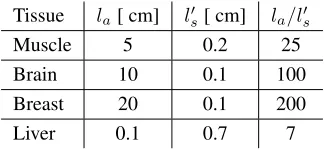
The diffusion approach generally assumes thatla l0s, that is, photons are scattered much more often

than they are absorbed. Jacques and Pogue22 showed that light transport in media withl0

s/la >20is very

well approximated with the photon diffusion equation. These limits apply to measurements of many tissues

with light in the NIR. For example, human breast tissue (la ∼20cm,l0s ∼ 0.1 cm) hasla/l0s ∼ 200at

∼800 nm (other tissues are shown in Table2.1).

The next few sub-sections will provide a mathematical underpinning for the analysis presented

through-out this thesis. Section2.2.1introduces notation. Section2.2.2briefly describes the derivation of the photon

diffusion equation from the radiative transport equation. Section2.2.3describes the diffusion equation for

photon fluence; Section2.2.4describes the accompanying boundary conditions. Several analytic solutions to

the diffusion equation for photon fluence in the Time (Section2.2.5) and Frequency (Section2.2.6) domains

Figure 2.2: Schematic of light scattering in tissue. Most individual scattering events (black) are strongly forward biased with scattering path lengthls∼10µm. However, many (∼100) of these forward scattering

events can be lumped together into a single, isotropic, event (red) with reduced scattering path lengthl0

s∼1

mm (blue). The absorption path length (not shown) in the diffusion regime is many timesl0

s.

Tissue la[ cm] l0s[ cm] la/l0s

Muscle 5 0.2 25

Brain 10 0.1 100

Breast 20 0.1 200

Liver 0.1 0.7 7

Table 2.1: Approximate Optical Properties in theNIRfor various tissues near 800nm. Note that liver isnot

(26)

are then described; these solutions are used in the analysis of Diffuse Optical Spectroscopy (DOS)

mea-surements. We then introduce Diffuse Correlation Spectroscopy (DCS; Section2.2.7) and Diffuse Optical

Tomography (DOT; Section2.2.8).

2.2.1 Diffuse Optical Notation

Diffusion models of photon transport are parameterized byla andl0s, the mean free paths for absorption

and isotropic scattering. However, in the Biomedical Optics Community, these models of photon transport

are typically written in terms of the inverses of the photon scattering lengths (i.e., the scattering coefficient,

µs= 1/ls, the reduced scattering,µ0s= 1/l0scoefficient, and the absorption coefficient,µa = 1/la).

If tissue had a single absorbing species, thenµa=C·[λ]. Here[λ]is the species wavelength dependent

extinction coefficient, andCis the species concentration. Scattering and absorbing cross-sections vary with

wavelength, and therefore bothµ0

sandµaare wavelength dependent. This notation is summarized in Table

2.2.

D Photon Diffusion Coefficient;D=₃₍_µ0v

s+µa), see Equation2.11[cm 2_s−1_].

g Anisotropy, mean cosine of scattering angle, see Equation2.7.

la Photon absorption length [cm].

ls Photon scattering length [cm].

l0

s Isotropicphoton scattering lengthls= (1−g)ls0 [cm].

µa Absorption coefficient, inverse of the absorption length,µa= 1/la[cm−1].

J[r,t] Photon flux, vector sum of radiance emanating from an infinitesimal volume centered atr, see Equation2.4[W cm−2].

L[r,Ωˆ, t] Light radiance atrandtin directionΩˆ, see Equation2.1and Equation2.2[W cm−2Sr−1].

µs Scattering coefficient, inverse of the scattering length,µs= 1/ls[cm−1].

µ0

s Reduced scattering coefficient, inverse of the isotropic scattering length,µ0s=µs(1−g)[cm−1]. Ψ[r] Photon fluence rate; angular integral of the radiance at positionr[W cm−2_].

Ref f Effective Fourier reflection coefficient from a diffuse non-diffuse boundary (e.g. tissue-air).

S[r] Isotropic source term; photons emitted per volume per time at positionr[W cm−3_].

v Speed of light in the medium [cm s−1_].

(27)

2.2.2 Approximation to the Radiative Transport Equation

Transport theory may be used to describe the propagation of light in tissues and other multiply scattering

media. The Radiative Transport Equation (RTE) is a conservation equation for radiance, i.e.,L[r,Ωˆ, t], the power per area traveling in directionΩˆ, [W cm−2 Sr−1] in an infinitesimal volume centered atr. (This description follows that in Durduranet al.25_{.) The RTE is given below.}

1

v

∂L[r,Ωˆ, t]

∂t + ˆΩ· ∇L[r,Ωˆ, t] =−µtL[r,Ωˆ, t] +Q[r,Ωˆ, t] +µs Z

4π

L[r,Ωˆ0, t]f[ ˆΩ,Ωˆ0]dΩˆ0 (2.1) Here, f[ ˆΩ,Ωˆ0_] _{is the normalized differential scattering cross section associated with a tissue scattering} (single-scattering) event (i.e., the probability of a photon traveling inΩˆ to scatter intoΩˆ0_); _Q_[_r_,_Ω_ˆ_{, t}_] _is the power per volume emitted by sources at positionrin directionΩˆ at time t, andvis the speed of light in the medium. The loss of radiance in an infinitesimal volume is dependent on the total attenuation coefficient

µt=µs+µa. The RTE describes photon transport under a wide range of conditions, but must be solved

numerically for most cases of interest. However, ifL[r,Ωˆ, t]is nearly isotropic (e.g., in a scattering medium far from the source), an expansion of the RTE in spherical harmonics truncated after the first term turns out

to be useful. This so-called P1 approximation (e.g., as in Case35_{) simplifies the radiance to}

L[r,Ωˆ, t] = 1

4πΨ[r, t] +

3

4πJ[r, t]·Ωˆ. (2.2)

Equation2.2introduces two terms describing photons emerging from an infinitesimal volume atrand time

t:

Ψ[r, t]_≡

Z

4π

L[r,Ωˆ, t]dΩ, (2.3)

the photon fluence rate (W cm−2, total power per area), and

J[r, t]≡

Z

4π

L[r,Ωˆ, t] ˆΩdΩ, (2.4)

the photon flux (W cm−2, vector sum of emitted radiance). Note thatJ[r, t]_·Ωˆ gives a power per area traveling in directionΩˆ.

Integrating Equation2.1over all solid angle results in an equation relatingΨandJ:

1

v ∂Ψ

∂t +∇ ·J[r, t] +µaΨ[r, t] =S[r, t]. (2.5)

Here we have introduced an ‘isotropic’ source termS[r, t] = R

Q[r,Ωˆ, t]dΩ(the total power per volume emitted at positionrand timet; W cm−3). Multiplying Equation2.1byΩˆ and substituting in Equation2.2

we arrive at

∇Ψ[r, t] =−_v3∂J_∂t[r, t]−3µtJ[r, t] + 3

Z

Q[r,Ωˆ, t] ˆΩdΩ + 3µsJ[r, t]

Z

4π

(28)

The rightmost integral in Equation2.6is an ensemble average of the cosine of the scattering angleθ

g_{≡ h}cos[θ]_i=

Z

4π

f[ ˆΩ,Ωˆ0] ˆΩ_·Ωˆ0dΩˆ0 (2.7) and defines the anisotropyg. As scattering in tissue becomes more forward scattering,gbecomes closer to

1;g∼0.7−0.99for most soft tissues38, 39_.

We next assume that we have isotropic sources, i.e.,

Z

Q[r,Ωˆ, t] ˆΩdΩ = 0, (2.8) and slow temporal changes inJ, i.e.,

1

v ∂J

∂t (µt−µsg)J. (2.9)

In this case, Equation2.6reduces to Fick’s law of diffusion:

∇Ψ[r, t] =₋3 (µa+µs)J[r, t] + 3gµsJ[r, t], =−3 (µa+µs(1−g))J[r, t], =₋3 (µa+µ0s)J[r, t],

∇Ψ[r, t] =₋v

DJ[r, t], (2.10)

where we have utilized the reduced scattering coefficientµ0

s≡(1−g)µsand defined the photon diffusion

coefficient

D_≡ v

3(µs+µa) '

v

3µs = vl

0

s

3 , (2.11)

sinceµa << µ0s.

With Equation2.10, Equation2.5becomes

∂

∂t− ∇ ·(D[r]∇) +vµa[r]

Ψ[r, t] =vS[r, t]. (2.12) Equation (2.12) is the time dependent photon diffusion equation for light in a medium with heterogeneous

optical properties under the assumptions noted above.

2.2.3 Time and Frequency Domain Diffusion Equation for Photon Fluence

For time-domain experiments, it is useful to consider the time domain diffusion equation with losses. The

diffusion equation for photon fluence rate (Equation2.12,Ψ[r, t], [W cm−2]) at a pointrand timetdue to an infinitely short, pulsed, isotropic point source at the origin(S[r, t] =S0δ[t]δ[r])is:

_∂

∂t− ∇ · D[r]∇

+vµa[r]

(29)

whereδ[x]denotes the Kroneker Delta Function forx.

For frequency domain analysis, it is convenient to separate the point source term into oscillating (ac)

and constant (dc) components:S[r, t] = Sdc+Sace−ıωt˙

δ[r]. Solutions to the diffusion equation (Equa-tion2.13) which oscillate at the same frequency will have the form

Ψ[r, t] =U[r]e−ıωt˙ _. _(2.14)

By substituting Equation2.14into Equation2.13, we arrive at

∇ · D[r]_∇

−(vµa[r]−ıω˙ )U[r] =−vSacδ[r] (2.15)

In a homogeneous medium, this reduces to

∇2

−k2

U[r] =₋v

DSacδ[r] (2.16)

with

k2=(vµa−˙ıω)

D . (2.17)

Note that the frequency domain diffusion equation has a general solution in the form of an over-damped

‘diffusive’ wave.

Boundary conditions are discussed in Section2.2.4; solutions in the time (Section2.2.5) and frequency

(Section2.2.6) domains are then presented in several important experimental geometries.

2.2.4 Boundary Conditions

The spatial boundary condition for an infinite medium is simple:Ψ_→0asr_{→ ∞}. However, this geometry has limited practical utility; various geometries used in practical experiments are discussed in Section2.3.2.

Here we will discuss the boundary conditions for ‘semi-infinite’ geometry (planar boundary between

clear and turbid half spaces). In the case of biomedical optics, tissue in air will typically be reasonably

well modeled as such a system; the resulting index of refraction mismatch will cause some photons to be

reflected from the boundary. The semi-infinite boundary conditions lead naturally into those for the ‘infinite

slab’ (two parallel planar boundaries) geometries; solutions using these conditions are utilized for the data

analysis presented in subsequent chapters.

In setting out the planar boundary conditions for the semi-infinite and slab solutions to the diffusion

equation, we will use a number of derived quantities to simplify notation; these quantities are summarized

in Table2.3.

Consider a turbid medium occupying an infinite half space. It is convenient to shift to cylindrical

(30)

z0=

1

µ0

s

zb= 2(l0s+la) 1 +Ref f 3(1₋Ref f)

z+,m= 2m(d+ 2zb) +z0

z−,m= 2m(d+ 2zb)−2zb−z0

r2

+,m=ρ2+ (z−z+,m)2

r2

−,m=ρ2+ (z−z−,m)2

z1,m=d(1−2m)−4mzb−z0=d−z+,m

z2,m=d(1−2m)−(4m−2)zb+z0=d−z−,m

r2

1,m=r2+,m[ρ, z=d] =ρ2+z12,m

r22,m=r

2

−,m[ρ, z=d] =ρ

2

+z22,m

k2

dos=

vµa

D

k2₌ vµa−ıω˙

D

Table 2.3: Notation used in describing semi-infinite and slab solutions to the diffusion equation in both time and frequency domain, wheremis the index of an infinite sum of dipoles used in the method of images,dis the thickness of the slab,zb is the extrapolated boundary condition (Equation2.30), andz0is the effective source position. r{1,2},m andz{1,2},msimplify notation when one is discussing transverse measurements

through a slab (i.e.,z=d).

Tissue

Air

Figure 2.3: Schematic of reflection of radiance (L[ ˆΩ]) off tissue-air boundary. The fraction of light reflected is the Fresnel coefficient (RF[ ˆΩ]); both quantities dependent on the input angle. nˆ is the surface normal;

ninandnoutthe indices of refraction in and outside the medium, respectively.

Assume input light impinges on the boundary in a narrow beam (e.g. from an optical fiber) at the origin.

This input light is generally well modeled as a point source at positionz0= 1/µ0sinto the medium.

Photons which exit the turbid medium are permanently lost. To determine the quantity of light which

reflects off the boundary, we return to the discussion in Section2.2.2and note that the photon flux into

(31)

direction:

Jin=

Z

ˆ Ω·n<ˆ 0

L[ ˆΩ] ˆΩ_·(₋nˆ)dΩ. (2.18)

Thus, at the boundary, all of the inward diffuse radiance is due to outward radiance reflected from the index

of refraction mismatch at the air-tissue boundary, i.e.,

Jin=

Z

ˆ Ω·ˆn>0

RF[ ˆΩ]L[ ˆΩ] ˆΩ·(ˆn)dΩ, (2.19)

whereRF[ ˆΩ]is the angularly dependent Fresnel reflection coefficient. By setting Equation2.18equal to

Equation2.19

Z

ˆ Ω·n<ˆ 0

L[ ˆΩ] ˆΩ·(−ˆn)dΩ =

Z

ˆ Ω·n>ˆ 0

RF[ ˆΩ]L[ ˆΩ] ˆΩ·(ˆn)dΩ.

Substituting in Equation2.2we arrive at:

Z

ˆ Ω·n<ˆ 0

₁

4πΨ[r, t] +

3

4πJ[r, t]·Ωˆ

ˆ

Ω_·(₋nˆ)dΩ =

Z

ˆ Ω·n>ˆ 0

RF[ ˆΩ]

₁

4πΨ[r, t] +

3

4πJ[r, t]·Ωˆ

ˆ

Ω_·(ˆn)dΩ.

(2.20)

The azimuthal angular dependence integrates out, leaving only the component in thezˆdirection:

1 4π

Z π/2 0

(Ψ[r, t] + 3Jz[r, t]cos[θ]) cos[θ] sin[θ]dθ, = 1

4π Z π/2

0

RF[θ] (Ψ[r, t] + 3Jz[r, t]cos[θ]) cos[θ] sin[θ]dθ. (2.21)

We define

RΨ= 2 Z π/2

0

RF[θ] cos[θ] sin[θ]dθ, (2.22)

RJ= 3 Z π/2

0

RF[θ] cos2[θ] sin[θ]dθ, (2.23)

and perform the angular integrals on the left side of Equation2.21, which can then be rewritten as

Ψ[r, t] 4 +

Jz[r, t] 2 =RΨ

Ψ[r, t] 4 +RJ

Jz[r, t]

2 , Ψ[r, t](RΨ−1) = 2Jz(1−RJ).

Thus, we can write the fluence rate as a constant times the flux at the boundary:

Ψ[r, t] = 1−RJ

RΨ−1

2JZ. (2.24)

From Equation2.10,

Jz=−

D v

∂Ψ

(32)

and therefore, at the boundary,

Ψ[r, t] = RJ−1

RΨ−1

2D v

∂Ψ

∂z. (2.26)

We then define an effective reflection coefficient forΨ

Ref f =

RΨ+RJ

2−RΨ+RJ

, (2.27)

and arrive at

Ψ[r, t] = 1 +Ref f 1₋Ref f

2D v

∂Ψ

∂z (2.28)

or more generally

Ψ[r, t] = 1 +Ref f 1₋Ref f

2D

v nˆ· ∇Ψ. (2.29)

Wherenˆis the surface normal as shown in Figure2.3. We then define an extrapolated boundary position:

zb =

1 +Ref f 1₋Ref f

2D

v (2.30)

and arrive at the typical formulation of the so-called partial flux or Robin boundary condition (which includes

boundary Fresnel reflection effects):

Ψ[r, t] =zbˆn· ∇Ψ[r, t]. (2.31)

While exact, the partial flux boundary condition is relatively difficult use in obtaining analytical solutions

to Equation2.13. However, if we perform a Taylor expansion on Equation2.31and truncate after the first

derivative term, we obtain a condition for which the fluence rate equals zero, i.e.,

Ψ[ρ, z=₋zb, t] = 0. (2.32)

This is the so-called extrapolated zero boundary condition40, 41_{; in this approximation, the fluence rate goes}

to zero in the plane parallel to the interface, but at a distancezb into the ‘air’ side of the interface. A

schematic of this extrapolated boundary is shown in Figure2.4.

Ref f, and thereforezb, is somewhat cumbersome to calculate, but can be well approximated by a

poly-nomial in the ratio of the indices of refraction. Contini42_writes_z

bas

zb= 2D

v A (2.33)

A= 1 +Ref f 1₋Ref f

(33)

Figure 2.4: Schematic of geometry for extrapolated zero boundary condition between air and tissue. The z-axis points into the medium. A narrow beam of light (red) impinges on the surface of the tissue. This light is modeled as a point sourcez0= 1/µ0sbelow the surface (red). An extrapolated boundary is placed at

−zband an image source at−(2zb+z0)(black dot); superposition of solutions from these sources produces

Ψ[zb] = 0.

and approximatesAas

A'504.332889−2641.00214n+ 5923.699064n2 −7376.355814n3_{+ 5507}_.₅₃₀₄₁_n4

−2463.357945n5_{+ 610}_.₉₅₆₅₄₇_n6

−64.8047n7+. . . (2.35)

forn= nin

nout >1(ninis inside the turbid medium andnoutoutside) and

A'3.084635−6.531194n+ 8.357854n2

−5.082751n3_{+ 1}_.₁₇₁₃₈₂_n4₊_{. . .} _(2.36)

forn= nin

nout <1.

With this effective zero fluence rate interface, analytic solutions to the diffusion equation (Equation2.13

and Equation 2.15) for the semi-infinite and slab geometries can be obtained using the solutions in the

infinite medium along with the method of images43, 44; the negative image source required for modeling a

semi-infinite boundary is shown in Figure2.4. A similar analysis for two interfaces can be applied to an

infinite slab. These solutions will be discussed in2.2.5and2.2.6. For these simple geometries, the Green’s

(34)

Collected

Light

Time

Input

Light

Figure 2.5: A schematic of a time domain measurement in an infinite homogeneous medium (i.e.,µaand

µ0

sare constants). A narrow input pulse is introduced into the medium (black dot, e.g. with an optical fiber).

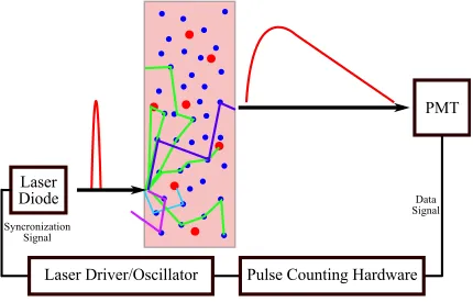
Photons scatter off the scattering centers (blue) and are absorbed by the absorbing centers (green). Most photons travel considerable distance from the input site; a few of these will arrive at a detector (gray dot, e.g., an collection optical fiber). As photons will travel many different paths to arrive at the detector, the input pulse is broadened by the time it reaches the detector.

2.2.5 Time Domain Solution to the Diffusion Equation

2.2.5.1 Solution to the Diffusion Equation in an Infinite Medium (Time-Domain)

The Green’s function for Eqn.2.13in an infinite homogeneous turbid medium (µa[r] =µa,D[r] =D) is:

G∞[r;rs, t] =

v

(4πDt)3/2e −|r−rs|2

4Dt −µavt _(2.37)

wherer=_|r_|, and the source is positioned atrs. NoteG∞→0asr→ ∞andt→ ∞. Figure2.5provides a schematic of this process for a source positioned at the origin. Real physical sources will have finite

spatial size and temporal width, and the fluence rate in these cases will be derived from a convolution of the

Green’s function with some spatial and temporal form characteristic of the source. In typical experiments,

the temporal form is measured; this measured signal is often called the ‘Instrument Response Function’

(IRF; discussed in detail in Section2.3.3) and included in the analysis by convolution with the solution for

an infinitely-short pulsed source.

Note that this analysis permits calculation of the average photon dwell time in tissue: G[r, t]describes a distribution function of photon arrival times due to a source at the origin and a detector atr. The time

(35)

directly for calculation of optical properties45_{. Arridge}46, 47_{has calculated these mean transit times (first}

temporal moments) for several geometries; Eqn.2.38, below, is the mean time for an infinite homogeneous

medium, whereris the displacement between the source and detector.

ht_i=1 2

|r_|2

D+_|r_|√µa·v·D

(2.38)

This mean transit time is sometimes converted into a Differential Path Length Factor (DPF) or Differential

Path length (DP) whereDP F = v_|h_rt_|iandDP =vhti(see also Sassaroli48).

2.2.5.2 Solution to the Diffusion Equation in a Semi-Infinite Medium (Time Domain)

In the semi-infinite geometry (Figure2.6), we apply the method of images to account for the boundary:

Gsemi−∞[r;rs, t] =G∞[r;rs, t]−G∞[r;r0s, t] (2.39)

wherer0_sis the position of the so-called image source.

Light is generally introduced into tissue using an optical fiber or a thin ‘pencil’ beam; for simplicity of

notation, we choose to place our input position at the origin (e.g., atρ= 0,z= 0orr= 0). This situation is well modeled by a point source displaced one reduced scattering path length into the medium (ρ = 0,

z=z0=ls0 orrs= [0,0, z0]); i.e.,

S[ρ= 0, z, t] =S0δ[t]δ[ρ]δ[z−zb]. (2.40)

This geometry is shown schematically in Figure2.6.

Utilizing this model for the source and the extrapolated zero boundary condition described in

Sec-tion2.2.4, we obtain

Gsemi−∞[r;rs, t] =G∞[r;rs, t]−G∞[r;r0s, t] (2.41)

Gsemi−∞[ρ, z;ρs= 0, zs=z0, t] =

v

(4πDt)3/2e −µavt

e−(z−z0 )2 +ρ 2 4Dt −e−

(z+z_{0 +2}zb)2 +ρ2

4Dt

(2.42)

wherer0_s= [0,0,₋(2zb+z0)](see Figure2.4).

Note, the analytical solution for the fluence rateΨfrom a source atrsof the formS =S0δ[t]δ[rs]is

simply

Ψ[r, t] =S0G[r;rs, t]. (2.43)

Combining the source term described in Equation2.40with the Green’s function solution to the diffusion

equation in Equation2.42, we can express the photon fluence rate in a semi-infinite mediumΨsemi−∞as

Ψsemi−∞[ρ, z, t] =S0

v

e−(z−z0 )2 +ρ 2 4Dt −e−

(z+z0 +2zb)2 +ρ2

4Dt

(36)

Input

Light

Collected

Light

Time

Figure 2.6: Schematic of semi-infinite (remission) geometry DOS, for a measurement on the input plane.

see Kienle49_{for additional details.}

Evaluating this expression on the clear-turbid (air-tissue,z= 0) interface results in

Ψsemi−∞[ρ, z= 0, t] =S0

v

e−z

2 0 +ρ2 4Dt −e−

(z_{0 +2}zb)2 +ρ2

4Dt

(2.45)

and measurable signal (power crossing the boundary or the integration over all possible photon angles exiting

the turbid medium a distanceρfrom the source)42_is

R[ρ, t] =D

v ∂

∂zΨsemi−∞[ρ, z= 0, t] (2.46)

= S0 2(4πD)3/2_t5/2e

−µavt

z0e− z2₀−ρ2

4Dt + (z₀+ 2z_b)e−

(z0 +2zb)2−ρ2

4Dt

(2.47)

2.2.5.3 Solution to the Diffusion Equation in an Infinite Slab (Time Domain)

Similarly, we can apply the extrapolated boundary conditions to a pair of parallel planar interfaces making

up an infinite slab (Figure2.7). Various derived quantities which permit simplification of the equations are

(37)

Input Light

Collected Light

Time

Figure 2.7: Schematic of infinite slab geometry DOS. A thin ‘pencil’ beam of light introduced to the tissue atρ= 0,z= 0is well modeled as a point source atρ= 0,z=z0∼ls0.

The Green’s function in such a slab with extrapolated boundary conditions, solved with the method of

images is42:

Gslab[ρ, z;ρs= 0, ρz= 0, t] =

ve−µavte− ρ

2 4πDt

2(4πDt)3/2

+∞ X

m=−∞

e−

(z−z₊_,m)2 4Dt

−

+∞ X

m=−∞

e−

(z−z−,m)2

4Dt

!

.

(2.48)

However, this solution does not yet describe the detected light (i.e., the radiance integrated over the

collection solid angle). Integrating over all possible photon angles existing the slab at a distanceρfrom the

source, the detectable light transmission can be shown to be

T[ρ, t] =₋D

v ∂

(38)

Detector

Source

Extrapolated

Boundary

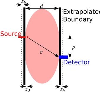
Figure 2.8: Compressed breast geometry (‘slab’).rdistance between source and detector,ρlateral (in plane) separation between source and detector,dplate separation,z0 = (µ0s)−1extrapolated source position, and

zbis the location of the extrapolated boundary.

Combining Equation2.43and Equation2.49, the transmitted light is described by

T[ρ, t] =S0e

−µavt_e− ρ

2 4πDt

2(4πD)3/2_t5/2 +∞ X

m=−∞

z1,me−

z₁2_,m

4Dt −z₂_,me− z2₂_,m

4Dt

. (2.50)

This expression usually is truncated after sufficient terms have been included to fit experimental data to the

required accuracy. Note that we have not yet included the finite temporal width of a physical source in this

expression; as mentioned above, this is accounted for by convoluting the solution for an infinitely short pulse

with the measured Instrument Response Function for a particular instrument.

Equation2.50can be integrated over time to provide the CW transmission as a function the transverse

distanceρ:

T[ρ] = S0 4π

∞ X

m=−∞ z1,m

r3 1,m

(1 +kdosr1,m)e−kdosr1,m

−z_r23,m 2,m

(39)

5

10

15

20

0

50

100 Time [ns]

Normalized Amplitude [%]

5

10

15

20

0.01

1

100 Time [ns]

Normalized Amplitude [%]

µ

s

′

= 10 cm

−1

ρ

= 0 cm

d = 6 cm

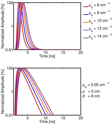
Figure 2.9: Graphs of Equation2.50for a slab withd=6 cm,ρ= 0cm,µ0s = 10cm−1, andµa as noted

in the legend. The amplitude for all the curves is normalized to show how longer photon paths (i.e., longer times) are suppressed as the absorption is increased.

This is the probability per unit area of a photon exiting the medium atρon the output plane. Examples of

(40)

5

10

15

20

0.01

1

100 Time [ns]

Normalized Amplitude [%]

5

10

15

20

0.01

1

100 Time [ns]

′

= 14 cm

−1

Figure 2.10: Graphs of Equation2.50 for a slab withd=6 cm, ρ = 0cm, µa = 0.05 cm−1, andµ0s as

(41)

5

10

15

20

0.01

1

100 Time [ns]

Normalized Amplitude [%]

5

10

15

20

0.01

1

100 Time [ns]

Normalized Amplitude [%]

µ

a

= 0.05 cm

−1

µ

s

′

= 10 cm

−1

d = 6 cm

ρ

= 0 cm

ρ

= 1 cm

ρ

= 2 cm

ρ

= 3 cm

ρ

= 4 cm

Figure 2.11: Graphs of Equation2.50for a slab withd=6 cm,µa =0.05 cm−1,µ0s = 10cm−1, andρas

Computer-Aided, Multi-Modal, and Compression Diffuse Optical Studies of Breast Tissue

University of Pennsylvania

ScholarlyCommons

Publicly Accessible Penn Dissertations

Fall 12-22-2011

Computer-Aided, Multi-Modal, and Compression

Diffuse Optical Studies of Breast Tissue

David R. Busch Jr

Follow this and additional works at:

http://repository.upenn.edu/edissertations

Part of the

Bioimaging and Biomedical Optics Commons,

Biological Engineering Commons,

Optics Commons, and the

Radiology Commons

Recommended Citation

Computer-Aided, Multi-Modal, and Compression Diffuse Optical Studies

of Breast Tissue

Diffuse Optical Tomography and Spectroscopy permit measurement of important physiological parameters

non-invasively through ~10 cm of tissue. I have applied these techniques in measurements of human breast

and breast cancer. My thesis integrates three loosely connected themes in this context: multi-modal breast

cancer imaging, automated data analysis of breast cancer images, and microvascular hemodynamics of breast

under compression. As per the first theme, I describe construction, testing, and the initial clinical usage of two

generations of imaging systems for simultaneous diffuse optical and magnetic resonance imaging. The second

project develops a statistical analysis of optical breast data from many spatial locations in a population of

cancers to derive a novel optical signature of malignancy; I then apply this data-derived signature for

localization of cancer in additional subjects. Finally, I construct and deploy diffuse optical instrumentation to

measure blood content and blood flow during breast compression; besides optics, this research has

implications for any method employing breast compression, e.g., mammography.

Dissertation

Doctor of Philosophy (PhD)

Physics & Astronomy

Arjun G. Yodh

diffuse optics, DOT, MRI, CAD, multi-modal imaging, compression, blood flow

COMPUTER-AIDED, MULTI-MODAL, AND

COMPRESSION DIFFUSE OPTICAL STUDIES OF

BREAST TISSUE

David Richard Busch Jr.

A Dissertation

Physics and Astronomy

c

Copyright 2011

Acknowledgements

ABSTRACT

Computer-Aided, Multi-Modal, and Compression Diffuse Optical Studies

of Breast Tissue

David Richard Busch Jr.

Arjun G. Yodh

Contents

List of Tables

List of Figures

Chapter 1

Introduction and Organization

Chapter 2

Introduction to Diffuse Optics

2.1

Introduction to Diffuse Optics

2.2

Mathematical Basis of Diffuse Optical Specroscopy &

Tomography

2.2.1

Diffuse Optical Notation

2.2.2

Approximation to the Radiative Transport Equation

2.2.3

Time and Frequency Domain Diffusion Equation for Photon Fluence

2.2.4

Boundary Conditions

Tissue

Air

Collected

Light

Time

Time

Input

Light

2.2.5

Time Domain Solution to the Diffusion Equation

Input

Light