Shape Function for Mesh Free Methods Using Moving Least- Squares Approximation Prof. Sanjaykumar D. Ambaliya , Prof. Pradip V. Savaliya

(1)

Shape Function for Mesh Free Methods Using Moving

Least-Squares Approximation

Prof. Sanjaykumar D. Ambaliya

*

, Prof. Pradip V. Savaliya

Department of Mechanical Engineering, Government Engineering College, Surat, Gujarat, India

ABSTRACT

Computational numerical simulation has increasingly become a very important approach for solving complex practical problems in engineering and science. Many of these approximate solution techniques are well-developed and possess much versatility in analyzing complicated phenomena whose behaviours is governed by increasingly complex partial differential equations. Among these approximate methods, the finite element method (FEM) is one of the most popular. Mesh free (MF) methods are among the breed of numerical analysis technique that are being vigorously developed to avoid the drawbacks that traditional methods like Finite Element method (FEM) possess. The main differentiating point between the meshfree and finite element methods is the shape function. The paper is intended to elaborate the construction of the moving least square (MLS) approximation shape function and their derivatives in one-dimension, by presenting the related plots of shape function and its derivatives; with different parameters. Element Free Galerkin (EFG) method is applied and results are obtained using MATLAB.

Keywords: FEM, EFG, MLS shape functions, Meshfree, Matlab

I.

INTRODUCTION

The development of the finite element method (FEM) in the 1950s was one of the most important advances in the field of numerical methods. The FEM is a robust and thoroughly developed method, and hence it is widely used in engineering fields due to its versatility for complex geometry and flexibility for many types of linear and non-linear problems. This mesh based numerical methods (FEM, FDM, CFD etc.) despite of great success; suffer from difficulties in some aspects, which limit their applications in many complex problems such as crack propagation, problems with phase change, large-strain deformations, etc. [1]

In recent years, meshless methods have been developed as alternative numerical approaches in efforts to eliminate known drawbacks of the finite element method (FEM). The main objective in developing meshless methods was to eliminate, or at least reduce, the difficulty of meshing and remeshing of complex structural elements. The nature of the various approximation functions employed by meshless methods

(2)

II.

METHODS AND MATERIAL

2. Moving Least-Squares (Mls) Approximation

There are a number of ways proposed to construct the meshfree shape functions [1]. In this paper the finite series representation, moving least square approximation method is studied. In 1981, Lancaster and Salkauskas formulated the Moving Least square approach [Lancaster, 1981]. Nayroles et al (1992) first used it for meshfree approximation and the idea was further formulated into EFGM framework by Belytschko et al (1994).

The Moving Least Square is widely used to generate the shape functions for various Mesh Free Methods. There are two salient Features of this method, firstly it creates a continuous and smooth approximation function in the field domain and secondly, the field function can be created with desired level of consistency. MLS involves the assumption of the field variable as a summation of series of monomials. The coefficients of the monomials are the unknowns and are calculated such that the squared sum of errors in the domain of a point is minimal. Once the approximation at a point is over, the MLS is „moved‟ to another point.

2.1 Meshfree shape function

The procedure for constructing the meshfree shape function using the MLS approximation starts with the assumption that x1, x2, x3 and xn are the nodes distributed in the domain Ω and the associated field variable or nodal parameter with these node are u1, u2, u3 and un. The approximated value of displacement function u(x) of a field variable defined on the domain Ω (0, 1) can be represented as,

( )

u x ≈

u

ˆ

(x) = 1

( ) ( ) ( ) ( ) m

T i i

i

p x a x P x a x





Where, P represents the polynomial basis function, m is the number of polynomial coefficients and a(x) is the unknown coefficient matrix.

The choice of the polynomial function is depends upon the basis and is decided by the Pascal‟s triangle. For example,

For 1-D problems,

PT (x) = [1, x], Linear m = 2

PT (x) = [1, x, x2], quadratic, m=3 and

( ) [ ( )

0 1

( )

2

( ) ,...

( )]

T

m

a x



a x

The unknown parameters a(x) at any given point are determined by minimizing the difference between the local approximation at that point and the nodal parameters ui. Let the nodes whose supports include xbe given local node numbers 1 to n. In order to determine the unknown coefficients a, a functional J is constructed. It sum up the weighted quadratic error for all nodes inside the support domain as

J = 1

ˆ

( )( )

n

i i

i

W x x u u



 



2

=

2

1

(

)(

( ) ( )

)

n

T

i i i

i

W x

x

P

x a x

u







Where n is the number of nodes in the neighbourhood of x for which the weight function, W(x — xi) ≠ 0, and ui refers to the nodal parameter of u at x = xi.

The polynomial basis and the weight function together cast a major influence on the performance of the MLS method. Then we want to minimize this functional, so we differentiate with respect to the unknown vector a(x), containing the coefficient,

J

a



= 0

By inserting the expression for J, the equation ends up with

2

1

(

( ) ( )

)

(

)

T n

i i

p x a x

u

J

W x

x

a



a











(3)

= 1

( )2( T( ) ( ) ) ( ) 0

n

i i i i

i

W x x P x a x u p x



  



= 1

( ) ( ) T( ) ( ) n

i i i

i

W x x P x P x a x

 



= 1 ( ) ( ) n

i i i i

W x x P x u







This can be written in a compact matrix form as,

( ) ( )

( )

A x a x



B x u

1

( ) ( ) ( )

a x A x B x u

Where,

1 1 1

1

(

) ( )

( )

n

T

I

A

w x

x P x P

x







1 2

1 2 2 2 2

1 1 2 2

1

1 1

( ) ( ) ... ( _n) n

n n

x

x x

w x x w x x w x x

x x

x x x x

     

  _ _  _ _  _ _

     

And,

B x( )[ (w xx P x1) ( ), (1 w xx2),... (w xx P xn) ( n)

1 2

1

1 1

( ) ( ) ... ( n)

n

w x x w x x w x x

x x x        _  _{ }  _{ }  _{ }_        

[

1, 2

,... ]

T

n

u



u u

u

The matrices A and B have been expanded above for the specific case of a linear basis in one dimension. By inserting this expression in, we get a new formulation of the displacement field,

1

( )

ˆ

T

( ) ( )

T

( )

( ) ( ) ( )

x

u

P x a x

P x A

x B x U x

 



= 1 ( ) ( ) n i i i

u x



x u





Where, the shape function is defined by,

1 1

1

( )

( )(

( ) ( ))

n

T

I I I

i

x

P x A

x B x

p A B



 







To determine the derivatives from the displacement, it is necessary to obtain the shape function derivatives. The spatial derivatives of the shape functions are obtained by,

1

,

(

),

T

I x

P A B

I x







1 1 1

(

P

T

,

_x

A B

 _I

P A

T

(



),

_x

B

_I

P A

T

(



) ,

B

_x





Where,

, 1

( )

(

) ( )

I x I

dw

B

x

x x p x

dx





1

,

_x

A

 _{is defined by,}

1 1 1

,

_x _x

A



 

A A A

 

Where,

1

1 1 1

1

,

(

) ( )

( )

n T x I

A



w x

x P x P

x









1 2

1 2 2 2 2

1 1 2 2

1

1 1

( ) ( ) ... ( _n) n

n n

x

x x

dw dw dw

x x x x x x

x x

x x x x

dx dx dx

 

   

  _ _  _ _  _ _

(4)

2.2 Weight Functions

The weights functions like cubic weight function, quartic weight, exponential weight etc, perform two actions, one as a medium of imparting smoothness or desired continuity to the approximation and other one, more important, is the establishment of the local nature of the approximation. The weight functions chosen for construction of shape function are as follows:

2

( / )

1

exp : ( )

0, 1

e fors

onential w s

fors

  

 _ 

 

   

 

 

Quartic spline:

3 4 4

1 6 8 3 , 1

( ) 0,

I I I I

I

i

s s s s

w s

s

     

  



 

Where, s= |x-xI|/dI and, dI is the radius of influence domain or radius of support domain of the node.

III.

RESULTS AND DISCUSSION

The various results related to behaviour of the shape function are presented along with the plots obtained using the MATLAB program.

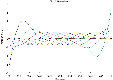
Figure 1: Shape function and derivative for cubic spline

2 3

2

1

4

3

2

4

1

:

( )

4

1

3

2

0,

s

s fors

cubicspline

w s

s

s for

s

for s























 





(5)

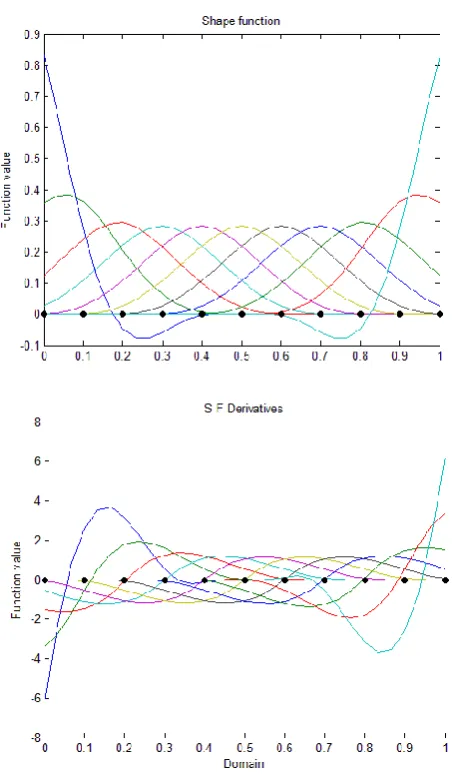
Figure 2 : Shape function and derivative for exponential function

Figure 3: Shape function and derivative for quartic spline

The effect of the basis function on the shape function is presented by figure. MLS shape functions using linear,

quadratic and cubic basis function and cubic spline weighting function are computed and plotted to visualize the effect of basis function on the shape functions. The study concludes that as the order of basis function is increased, the value of shape function is increases to maximum and becomes constant as the order of basis and weighting function become equal.

Figure 4 : Shape function with different basis functions

The table-1 presents the values of shape function associated with for the middle node (node number five) at x = 0.5. It shows that the shape function approximates and satisfies partition of unity conditions subject to use of constant terms.

Also, the value of shape function at node 5 is = 0.3807 ≠ 1.0. Thus the moving least square shape functions do not satisfy the Kronecker delta condition.

IV.

CONCLUSION

(6)

The selection of the weighting function plays a very vital role in the formulation and solution of meshfree methods. It is concluded that the cubic spline weighting function gives the shape function which possess more local character. The shape function inherits the features of weighting functions like shape and order of continuities.

The shape functions possess the bell shape, presented in figure-1 through 3, as the number of nodes in the support domain is increased the height of the bell gets lowered and spread gets lengthened increasing the global influence.

V.

REFERENCES

[1]. Liu G. R., 2004, “Mesh Free Methods: moving beyond the finite element method”, Ed. CRC Press, Florida,USA,

[2]. T. Belytschk O, Y.Y.Lu And L.GU, "An Introduction to Programming the Meshless Element Free Galerkin Method" International journal for numerical methods in engineering, VOL. 37, 229-256 (1994).

[3]. T. Belytschko,Y. Krongauz, D. Organ, "Meshless Methods: An Overview and Recent Developments" May 2, 1996.

[4]. J. Dolbow, T. Belytschko, "Numerical integration of the Galerkin weak form in meshfree methods" Computational Mechanics 23 (1999) 219-230 Ó Springer-Verlag 1999.

[5]. S. D. Daxini and J. M. Prajapati, "A Review on Recent Contribution of Meshfree Methods to Structure and Fracture Mechanics Applications" Scientific World Journal Volume 2014, Article ID 247172, 13 pages

[6]. J. Dolbow, T. Belytschko, "Numerical integration of the Galerkin weak form in meshfree methods" Computational Mechanics 23 (1999) 219-230, Springer-Verlag 1999.

[7]. "An Introduction to Meshfree methods and their Programming" by G.R. LIU, 2005.

[8]. "From Weighted Residual Methods to Finite  Element Methods" by Lars‐Erik Lindgren, 2009. [9]. "Meshfree and Generalized Finite Element

Methods" by Habilitationsschrift, 2008