Published online February 20, 2013 (http://www.sciencepublishinggroup.com/j/ijssn) doi: 10.11648/j. ijssn.20130101.11
Meeting the challenges for wireless sensor network
deployment in buildings
Costas Daskalakis, Nikos Sakkas, Maria Kouveletsou
*Applied Industrial Technologies Ltd., Gerakas, Attiki, Greece
Email address:
[email protected] (C. Daskalakis), [email protected] (N. Sakkas), [email protected] (M. Kouveletsou)
To cite this article:
Costas Daskalakis, Nikos Sakkas, Maria Kouveletsou. Meeting the Challenges for Wireless Sensor Network Deployment in Buildings,
International Journal of Sensors and Sensor Networks. Vol. 1, No. 1, 2013, pp. 1-9. doi: 10.11648/j.ijssn.20130101.11
Abstract:
Wireless sensor networks (WSNs) in buildings are faced with transmission issues, much more severe than those of outdoor applications. Next to the transmission effective range, battery lifetime is also of a high importance, as it can sig-nificantly affect network performance and maintenance requirements. In this paper we present an architectural concept, in fact a dynamic routing protocol, for the setup of a building WSN. Three key goals have underpinned the protocol design; ability to cost efficiently address transmission distance within buildings, acceptable battery longevity, typically up to a year, and no data loss. Experimental data have been collected over a period of several months and have demonstrated the much enhanced performance of the network, when compared to the performance before the protocol implementation.Keywords:
Wireless Networks, Dynamic Routing, Relaying1. Introduction
In the framework of an EU research program [1], an ad-vanced energy monitoring and control system was planned for installation in a three floor, plus basement, building. This system would be based on a wireless sensor network (WSN). The WSN would be deployed with the aim to pro-vide for energy management as well as for a joint and real time view on energy consumption and the respective indoor environment quality. Indoor installations of wireless net-works present many challenges, primarily in terms of transmission effective ranges as well battery lifetime and, consequently, network, maintenance free, operation.
The pilot building had an overall height around 12m and an average surface area of about 640 sq. m. The building volume was approximately 1000 cubic meters. Load bear-ing elements had been constructed from reinforced concrete, and had a typical thickness 25- 30 cm; bricks, synthetic panels, etc, had been used as non load bearing structural elements. Cooling was based on heat pumps; because of the passive architectural elements used, cooling needs were minimal; ventilation was purely natural and no mechanical means had been installed.
The project was planned for completion by early 2013. At the moment of the paper preparation (2012), work is still in progress; a number or wireless nodes have been installed in the building, and sensors have been linked to them;
sen-sor-boards deployed till now monitor electric energy as well as environmental parameters and occupancy; thermal energy and water temperature sensors nodes will follow in the next months.
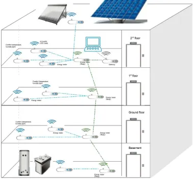
The network planned for installation in this building will be gradually deployed all across it, and will monitor ap-proximately 25- 40 electric and thermal energy consump-tion, storage and production points. Thermal and PV panels have been deployed on the building roof as energy produc-ers. In the basement, a hot water boiler and a battery pack provide for thermal and electric, respectively, energy sto-rage. The network will also monitor environmental condi-tions such as temperature, humidity, CO2, in order to pro-vide for a correlation between the energy used in particular building spaces (offices) and the quality of the environ-ment.
The nodes that have been currently deployed are located in all three floors as well as the basement and the terrace. The network gateway, which collects all the sensor data, is on the top floor. The gateway node communicates with an application that then sends the data to a web server where they are published real time. Network nodes have distances ranging from 2 m to 25 m from this gateway node.
2. Background and Motivation
al-low monitoring devices, user and building performance, calculating respective performance indicators and issuing advice for the building user. To also support several control operations of the renewable energy infrastructure.
The network was based on wireless nodes [2] pro-grammed on TinyOS [3, 4]. A number of known architec-tural approaches, such as single-hop transmission and the Collection Tree Protocol (CTP) [5], implemented for the TinyOS, were initially used, which however did not perform well in terms of the above criteria. The problems manifested as significant data loss due to frequent instances of com-munication loss, as well as a rapid deterioration of battery performance.
To address these issues, a dynamic routing architecture has been designed and the wireless sensor network has been respectively programmed. Similar routing techniques have been introduced [6] which do not have the drawbacks of CTP. Another type of routing protocols, known as position based routing [7] exist, but they usually include a Global Position
System (GPS) module, which is not acceptable due to in-creased energy consumption and specific operating condi-tions (open space).
The routing was somehow designed with the nature of the application context in mind; energy management in build-ings. Because of this particular context, it has been safe to assume that there would, by definition, be a number of points were electric energy would be monitored. These wireless nodes, obviously battery independent, would then assume a special, relaying role in the transmission archi-tecture. Therefore, although several of the concepts used can be relevant also in outdoor environments, where network nodes may not be easily sourced by electricity, the archi-tecture and routing relevance is far greater in the case of indoor applications, which assumes that certain nodes may be mains powered.
3. The Deployed Wireless Network
Figure 1. WSN Topology.
The wireless nodes have been based on the TinyOS technology and have been provided by MaxFor (Korea) and SowNet (Netherlands). In the former case, the operation frequency was that of 2.4GHz; in the latter 800MHz. Dep-loyed nodes have been equipped with either an on board or an external antenna. Each node has been connected to one or
developed on the ADE chip (Analog Devices ADE7753 chip). The current sensing element was of a shunt type; the sensors were capable of measuring one phase current up to 20 A. Further sensors are now being developed on the same chip for higher currents as well as three phase currents. A special type of a, so called, occupancy sensor board has also been deployed in several spaces (rooms, etc.). This board is based on the Murata PIR (pyro-electric infrared) sensor, typically used for human presence detection. The occupancy board, however, does not just sense presence. It has been designed as to discern between humans entering and exiting spaces and, in this way, provides real time values for space occupancy. Such values can then be used to develop a new generation of actual-data based energy efficiency indicators. Space energy consumed can then be related with actual occupancy, i.e., the serviced population, and not just with space surface or theoretic populations, as typically the case. Fig. 1 below broadly illustrates the WSN topology.
4. Problems Encountered
Two types of problems were encountered from the very first trials. First, despite the relatively small distances (maximum 25m) because of the indoor nature of the instal-lation the nodes would often loose communication with the base gateway. Second, batteries, in several cases, were
ex-hausted in a matter of weeks. To address these issues a number of routing provisions were made [8]. These will be briefly discussed below.
4.1. Addressing the Limited Battery Life
Initially, the single-hop transmission was attempted, where nodes transmitted the data directly to the gateway. This approach is very simple in concept and very effective in terms of battery lifetime, but is the least flexible and doesn't allow for nodes to be deployed far from the gateway. The shortcomings of the approach and its inability to chal-lenge the required distances, very soon became apparent. As a next option, the well established CTP was used. In this approach, nodes were constantly listening for incoming requests, which they then forwarded to the next listener and so on, till the data reached the gateway. This approach is flexible, results, however, to a fast degradation of the net-work performance; listening, unfortunately, comes at an energy cost that appeared detrimental in terms of battery lifetime [9].
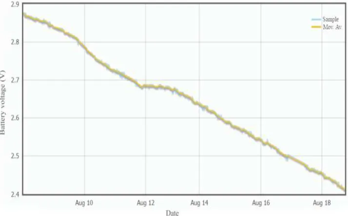
Fig. 2 shows the performance of a node with an external antenna, with a sampling rate of 30 sec. The battery was exhausted in as little 10 days! A voltage below 2.5V will not transmit reliable data.
Figure 2. Battery performance for a node with external antenna, with a sampling rate of 30 seconds.
The approach that yielded the most promising results in addressing the limited battery lifetime issue was the adop-tion of an energy efficient, communicaadop-tion protocol. This protocol required that radios remained switched off and were active only during the transmission of the data to the gateway. Obviously, we had to completely depart from any radio "listening" concept as this resulted to a rapid decrease of the network performance [10].
Initially we opted for a fixed configuration; nodes
communication protocol, where nodes were most of the time in the energy optimal state of sleep, increased the per-formance by an order of magnitude.
Fig. 3 shows a node deployed in an office. Now the
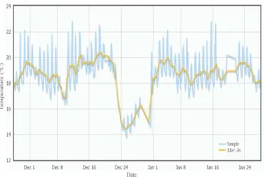
bat-tery remains in operation after two months, well above the critical operation voltage (~2.55 V) even during stressful conditions. On Fig. 4 the temperature variation in the pe-riod is displayed.
Figure 3: Battery remains in operation after two months.
Figure 4. Temperature variation for the same period.
Obviously the sampling rate has a significant impact on such a configuration. The less often sensors are sampled, the less the radio needs to wake up. We did implement a number of sampling rates (between 30 and 300 sec) which fully justified this view. This, in addition with a possible removal of the unnecessary and energy consuming external antenna and its substitution with an on-board, more energy
efficient variant, would bring the battery longevity close to a year.
4.2. Data Loss Issues
which data are able to automatically find a way to the ga-teway, provided no distance between two nodes is far too big to communicate the data across.
In our network implementation and despite the relatively small distances (maximum 25m) it was not always possible to reach directly the gateway; even more we noticed that this was not always an on/ off situation; often the node lost communication to the gateway which it resumed however at later moment. In the meanwhile, however, data read from the sensors during the non communication period, were lost. The second reason of data loss incidents was related to In-ternet connectivity issues. As the network serves a web application and transfers its data to a web server database, every loss of internet connectivity resulted also to data loss. Finally, data loss could arise due to a failure of the PC hosting the gateway, or due to a power disruption, exceed-ing its UPS capacity. This is the case illustrated in fig. 3 and fig. 4, for several days between end of July and begin-ning of August. This was a power failure of the gateway PC in a period where offices were shut due to vacations.
Thus, we had to address two important situations. First, to provide a solution for those nodes who, due to distance, would never be able to directly reach the gateway, without resorting to the energy inefficiencies of CTP [11]; second to provide a solution to prevent data loss, in all situations as those described above.
4.2.1 Relaying
By the very purpose of our network, it will always in-clude a number of electric meter nodes, measuring electric energy and power on a number of locations (devices, cabi-nets, etc.).
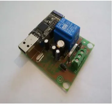
Fig. 5 illustrates a prototype electric energy sensor (the Analog Devices energy sensing chip is on the back side). Such sensors were installed in a cabinet to monitor space consumption or near devices to monitor, for example, cooling heat pumps, heaters, washing machines, burners etc.
Figure 5. Electric sensor used as a relay node.
Such nodes do not need any battery and do not have any respective energy limitations; instead of programming
those to be, by default, in sleep mode, they can be, at no performance cost, on the alert. Thus, we can use these nodes as, so called, data relaying nodes. They offer a good, energy wise, pathway for data transmission, for those re-mote nodes, not directly reaching the gateway. Making use of such nodes and assigning them this special relaying role will solve the effective distance problem of the remote nodes. Of course, similar may apply in environments were no mains fed energy sensors are used. Any sensor board, which can in fact connect to the mains, is a candidate for assuming a relaying role. However, convenience dictates that should energy metering be part of the set-up, these wireless meters are the best and most convenient candidates for relaying data.
4.2.2 Data Routing and Buffering
Before presenting the dynamic routing protocol we will illustrate the key network functionality in a more static and preconfigured setup. In fact, this was the first step to ad-dress the key issues of our concern. As soon as the functio-nality was proven, then the dynamic, ad-hoc features of the network were implemented, resulting to a flexible and completely dynamic routing protocol.
A first requirement was to embed in the design some contingency. If a specific path could not, for any reason, transmit the data, then a second option should be tried. Fig. 6 illustrates two such alternative paths programmed for a sensor node; one (primary) via a relaying node and one (secondary) directly to the gateway. It is again emphasized that these two paths, are, for now, hardwired; later they will result as part of the dynamic routing protocol.
Here is how the setup works: The node is most of the time in a sleep mode, until its timer wakes it up (wake-up mode) to sense the data it has been assigned to. After the data are sensed the node seeks to transmit them via its pri-mary path, leading, in this example, to a relay node. The relay node may truly receive them and dispatch an ac-knowledgment, mission complete, signal to our node, which then enters again its sleep mode. If however the re-lay node, for any reason, will not acknowledge data recep-tion then the node will try its second transmission path, in this example, by sending directly to the gateway. A similar acknowledgment process is executed. It the gateway con-firms data reception then the mote goes safely in its sleep mode. If, however, again the mote does not receive the ac-knowledgment then it will start buffering the data to its local memory. Buffering offers a means to avoid data loss. As we will see, as soon as the problem, whatever it may be, is removed, the mote will offload all its locally saved data to either of its target motes, starting from the default one (the relaying node).
When this happens, and an acknowledgment signal is eventually received, then operation will be back to normal, the local memory will be flushed and the mote will again go in its sleep mode. The local memory size and the
sam-pling rate will define how long the node may store its data locally, with no data loss. In our case this has ranged be-tween several months and a year!
Figure 6. Sensor node; 3 modes (sleep, wake, buffer), 2 paths.
By providing these alternative paths we were able to re-program two of the nodes deployed, which experienced transmission problems and data loss. Fig. 7 and Fig. 8, and
in particular the horizontal segments illustrate such cases of data loss due to loss of contact.
Figure 8. Data loss from noon 11 July till noon 12 July; connection restored thereafter.
Their preferred transmission path was now via energy meter relaying nodes that were located more closely to them. As explained above, a buffering concept was also programmed to address data loss.
Through this buffering provision, all data loss that was observed previously to this implementation was completely
resolved and the robustness of the network considerably increased.
Fig. 9 shows the performance of a sensor node with buf-fering implemented. Horizontal segments, indicative of a communication loss, are no more the case.
Figure 9. Sensor node with buffering implemented; no data loss experienced.
4.3. Time Stamping the Data Samples
When read, sensor samples need to be time-stamped. Nodes do not have any real time clock (RTC) to time-stamp the samples precisely. At the single-hop case, where data are transmitted directly to the gateway and no data buffer-ing is takbuffer-ing place, we can safely assume that the time of the sampling is the time the data reaches the gateway and the PC. All PCs obviously are equipped with RTCs. At the current case, where relaying nodes are used and buffering might occur at any time, delaying the data in reaching the gateway, this assumption cannot stand.
Every node, since it includes a microprocessor, has an internal clock which can be used to measure the time
elapsed since the boot-up of the node. Although it doesn't provide an absolute, real time, it can provide a relative time. In TinyOS, there is an implementation of TimeSync [12], where the local time of each node is synchronized with the RTC of the PC and the gateway connected to it. This me-thod seems to be very poor energy-wise, as it needs a radio communication in short intervals to synchronize the clocks. Also, depending on the network topology, it might take several minutes until all the nodes are synchronized [13]. A simple concept of TimeOffset was introduced to timestamp the data samples. This method uses only the local clock of each node to help determine the real time of the sampling, without any need of time synchronization.
stamped with the local time of the node. Then, the sample is transmitted to the next node with the difference between the sampling time and the transmitted time. If this trans-mission happens immediately, then the time-offset is 0. If for some reason the transmission is not successful and is retried at a later time, then the time-offset will be that time difference. The next node will receive the sample and will timestamp it with its own local time, keeping the previously time-offset from the previous node too.
Again, the sample will be transmitted to the next node with the time offset between the time received and the time transmitted plus the previous time offset. Eventually, the sample will reach the gateway and the PC with a total time offset between the sample time and the receive time. Sub-tracting this time offset from the local real time of the PC, will result to a very precise and absolute time-stamp of the sample.
5. Dynamic Routing
We will now investigate how the above relaying, buffer-ing, etc., principles were integrated in a dynamic routing protocol that allowed the network to fully self configure its communication path [14]. It is interesting to note that compared to the above static routing configuration, in the dynamic routing the requirement for the two, alternative, fixed paths, was not any more in place. We will explain this automatic configuration process, by looking in how every new node was accommodated in the network.
Every new node entering the network needs first to iden-tify a parent. Before a transmission of a sample, the node checks if there is a parent defined. If there is no parent de-fined, the node will broadcast a “request for parent” mes-sage and will wait one second for responses. All nodes in radio range, which succeed in receiving the “request for parent” message and have a parent different from the re-questing node, will respond by sending back a “request for parent response” message with a random delay (0-500ms). The random delay was introduced to minimize the possibil-ity of colliding response messages.
The node will now construct a list including the nodeID and the RSSI value, for every candidate parent. RSSI cor-responds to the received signal strength indicator and is a measure of the power present in a received radio signal. From this list, the best candidate is chosen as parent, by means of the best RSSI and is assigned as the node paren-tID parameter.
Every node which is assigned as a parent will construct a childlist table. This table consists of pairs [childID → pa-rentID]. When a node sends a sample to its parent it in-cludes in the message the respective [childID → parentID] pair.
5.1. An Example of Dynamic Routing
The following example demonstrates how the childlist table is constructed.
Fig. 10 illustrates a network comprising 9 nodes, among
which a gateway (Node 0), connected to a PC. The network has been gradually set up according to the above presented process. Let us now see how the data transmission will oc-cur and what exactly will be, every time, transmitted. Let us assume Node 7 as the start node.
Figure 10. WSN topology; dynamic routing.
When node 7 will wake up, it will transmit to its parent node 3 its sample along the pair [7→3]. This pair is stored on the node 3 childlist. Node 3 will forward this sample to its own parent, node 5. Then, node 5 will also store to its childlist the same pair [7→3]. Likewise, node 5 will forward the sample to its parent, node 1, along the pair [7→3], which again updates the childlist of node 1. Finally, node 1 will forward the sample to node 0. The same process is applied to every node, when it transmits its sample to its parent, in order to reach the gateway.
This childlist provision is crucial in order to support cases, where the gateway needs to send a message to a specific node or when a node needs to communicate directly with another node. There are certain cases where data from a given node need be transferred to another node to support some control action carried out at that point. One of the purposes of the dynamic routing presented here is to allow for such a clear and unambiguous transmission path between any node pair.
With regard to the above example, Table 1 below shows the childlist table of every node, constructed in the above mentioned way.
the update and will realize the change (its Childlist has changed! and in particular a parent-child relationship has changed!). It will then broadcast a message communicating to all nodes the change in its Childlist structure. The gateway will take no action in cases on new nodes. It will update its Childlist but there is now no need to broadcast anything. The above process applies to changes in the [child, parent] rela-tionship and not when a new node is introduced.
Table 1. Parent- Childlist table.
NodeID ParentID Childlist
ChildID ParentID
7 3 - -
4 3 - -
8 2 - -
3 5 7 3
4 3
2 1 8 2
5 1
3 5
7 3
4 3
6 1 - -
1 0 8 2
0 -
7 3
4 3
3 5
2 1
5 1
6 1
8 2
7 3
4 3
3 5
2 1
5 1
6 1
1 0
6. Conclusions
Building level WSN applications are faced with signifi-cant challenges as regards transmission range, battery lon-gevity and data loss.
An architectural concept has been implemented on a Ti-nyOS WSN that has allowed to successfully addressing such requirements, by eliminating data loss and securing battery lifetimes up to a year. This overcomes the problems asso-ciated with the CTP meshing protocol, which has not been found to be an optimal approach in the building context, because of its energy inefficient characteristics.
Besides the static, node level, concepts, such as relaying and data buffering, the architecture includes also a dynamic routing protocol that allows the network to self configure, define its optimal transmission paths and assume instant corrective actions whenever a node enters or exits the net-work. Ad hoc communications can be thus optimally achieved, not only between a node and the gateway but also
reversely, between the gateway and a node as well as be-tween any pair of network nodes. This has been found a very useful feature for building applications where data from a given node need be transferred to another node to be used in decentralized control operations.
References
[1] EnergyWarden, 2010, European Commission, 23 Jun 2012 http://energywarden.net.
[2] Karl H. and Willig A. (2007) Protocols and Architectures for Wireless Sensor Networks. England: John Wiley & Sons.
[3] Levis P. and Gay D. (2009) TinyOS Programming. United Kingdom: Cambridge University Press.
[4] TinyOS, 2011, University of California Berkeley, 23 Jun 2012 http://www.tinyos.net.
[5] Gnawali O., Fonseca R., Jamieson K., Moss D., Levis P., Collection tree protocol, Proceedings of the 7th ACM Con-ference on Embedded Networked Sensor Systems (2009) 126-127.
[6] D. B. Johnson and D. A. Maltz, Dynamic Source Routing in Ad-Hoc Wireless Networks, Mobile Computing (1996).
[7] Sinchan R. and Chiranjib P., Geographic Adaptive Fidelity and Geographic Energy Aware Routing in Ad Hoc Routing, Special Issue of IJCCT Vol.1 Issue 2, 3, 4; 2010 for Interna-tional Conference [ACCTA-2010], 3-5 August 2010.
[8] Gelenbe E., Lent R., Power-aware ad hoc cognitive packet networks, Ad Hoc Networks 2(3) (2004) 205-216.
[9] Wattenhofer R., Li L., Bahl P., Wang Y.-M., Distributed topology control for power efficient operation in multihop wireless ad hoc networks, Proceedings of INFOCOM 2011, Twentieth Annual Joint Conference of the IEEE Computer and Communications Societies, IEEE 3 (2001) 1388-1397.
[10] Mhatre V., Rosenberg C., Design guidelines for wireless sensor networks: communication, clustering and aggregation, Ad Hoc Networks 2(1) (2004) 45-63.
[11] Qiu W., Skafidas E., Hao P., Enhanced tree routing for wireless sensor networks, Ad Hoc Networks 7(3) (2009) 638-650.
[12] Maroti M., Kusy B., Simon G., Ledeczi A., The flooding time synchronization protocol, Proceedings of the 2nd in-ternational conference on Embedded networked sensor sys-tems (2004) 39-49.
[13] Sundararaman B., Buy U., Kshemkalayani A.D., Clock synchronization for wireless sensor networks: a survey, Ad Hoc Networks 3(3) (2005) 281-323.