http://www.sciencepublishinggroup.com/j/jeee doi: 10.11648/j.jeee.20200801.11
ISSN: 2329-1613 (Print); ISSN: 2329-1605 (Online)
A Schmitt Trigger Based Oscillatory Neural Network for
Reservoir Computing
Ting Zhang, Mohammad Rafiqul Haider
*Department of Electrical and Computer Engineering, University of Alabama at Birmingham, Birmingham, the United States
Email address:
*
Corresponding author
To cite this article:
Ting Zhang, Mohammad Rafiqul Haider. A Schmitt Trigger Based Oscillatory Neural Network for Reservoir Computing. Journal of Electrical and Electronic Engineering. Vol. 8, No. 1, 2020, pp. 1-9. doi: 10.11648/j.jeee.20200801.11
Received: November 15, 2019; Accepted: December 2, 2019; Published: January 4, 2020
Abstract:
With the increase in communication bandwidth and frequency, the development level of communication technology is also constantly developing. The scale of the Internet of Things (IoT) has shifted from single point-to-point communication to mesh communication between sensors. However, the large sensors serving the infrastructure place a burden on real-time monitoring, data transmission, and even data analysis. The information processing method is experimentally demonstrated with a non-linear Schmitt trigger oscillator. A neuronally inspired concept called reservoir computing has been implemented. The synchronization frequency prediction tasks are utilized as benchmarks to reduce the computational load. The oscillator's oscillation frequency is affected by the sensor input, further affecting the storage pattern of the oscillatory neural network. This paper proposes a method of information processing by training and modulating the weights of the intrinsic electronic neural network to achieve the next step prediction. The effects on the frequency of a single oscillator in a coupled oscillatory neural network are studied under asynchronous and synchronization modes. Principle Component Analysis (PCA) is used to reduce the data dimension, and Support Vector Machine (SVM) is used to classify the synchronous and asynchronous data. We define that oscillator with stronger coupling weight (lower coupling resistance) as a leader oscillator. From the spice simulation, when OSC1 and OSC2 work as leader oscillator, the ONN almost always achieve synchronization; and the synchronization frequency isclose to the average value of the leader oscillators. By training the emerging synchronous and asynchronous data, we can predict the synchronization status of an unknown dataset. Weight retrieval can be achieved by adjusting the slope and bias of the separation boundary.
Keywords:
Schmitt Trigger Oscillator, Reservoir Computing, Coupling Weight, Synchronization Frequency1. Introduction
Recent trends in information processing place high demands on a complex dynamical system in a small area and still reduce power consumption [1-5]. Since the 1980s, with
the development of Complementary
metal-oxide-semiconductor (CMOS) technology, the convergence of learning rules and very large scale integration (VLSI) technologies, the size of the device channel has entered a dozen or even a few nanometers and transistor integration density has grown tremendously which made it is possible to simulate the nervous system better to validate the model and cultivate new biologically inspired ideas [6]. Considering the limitation of improvement in CMOS technology on device scaling, memory capacity, and power
weights and freely connected neurons in the reservoir layer, theoretically, any complex non-linear system can achieve infinite approximation, which makes it possible for the complex net-works to perform computation efficiently [14]. One of these concepts is known as Echo State Network by Wolfgang Maass [15] and Liquid State Machine by Herbert Jaeger [16] or more generally as a neurally inspired referred to as Reservoir Computing for non-linear system identification, prediction, and classification.
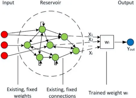
For general neural networks, we start adapting the weight of all the connections when we are training the weight [17], in which the training process is very difficult for non-linear complex dynamical systems [18]. However, in reservoir computing, we are going to have random, fixed weight connections. Instead of changing the existing connections, we fit the existing weight connection in the reservoir layer by changing the weight connection between the reservoir layer and the output layer. The benefit of training the weight externally is that we can substitute the existing system to another system that fulfills the specific property. The training makes it possible to solve the problem of the complex dynamical system, which poses non-linearity and high-dimensional mapping. However, in the real world, non-linear oscillators are more usual than linear cases [19]. While the hysteresis of the Schmitt trigger oscillator is challenging to take account in a theoretical model, reservoir computing provides a workable approach for realizing pattern recognition by analyzing the properties of synchronization of the Schmitt trigger oscillators.
In this paper, we demonstrate the nanoscale frequency storable oscillator using Schmitt trigger with resistive sensor devices connected in bus topology to store information as an oscillation frequency. We implement an input signal and feed it into a fixed dynamical system called a reservoir and the dynamics of the reservoir map the input to a higher dimension. Then the weight is trained to read the state of the reservoir and map it to the known output, further predict the unknown output.
2. Reservoir Computing
Reservoir Computing, also known as the Echo state network, is considered an extension of the Neural Network. A reservoir computer consists of the following three parts: an input layer, reservoir layer, and output layer. Input layer: it can be composed of one or more nodes and belongs to a kind of feed-forward neural network. Reservoir layer: consists of multiple nodes belonging to the recurrent neural network. Output layer: a weighted summer. Figure 1 shows the most general case of the reservoir computing schematic. In which
∑ (1)
In our reservoir computing architecture, the input layer is
providing an input signal to our reservoir. There are different input channels so that we can send a different input signal to our actual oscillatory neural network. The reservoir layer is a network of recurrently and randomly connected nonlinear
nodes [21-22]. It is for transforming the non-linearly separable to linearly separable. The difference between the input layer and the reservoir layer is that the former only allows signals to pass from the input layer to the output layer. The signal transmission is unidirectional, and there is no loop at all. The output of any layer cannot be data that affects the layer itself and is therefore typically used for pattern recognition. On the other hand, by introducing loops, the signals could be allowed to pass in both directions. The output layer is the layer we are training.
The advantage of reservoir computing is that the middle layer's reservoir connection is randomly generated and remains unchanged after it is generated. We only need to train the weight in the output layer, which makes it much faster than the traditional method. This is a unique part of reservoir computing.
Figure 1. Schematic of Reservoir Computing Architecture.
3. Application to Electronic Networks
There is a wide choice of designs for electronic oscillators [23]. Since non-linear oscillators are more usual than linear cases, a Schmitt trigger oscillator is used as CMOS neuron in our oscillatory neural network circuit to perform as a non-linear oscillator.
3.1. Introduction of Schmitt Trigger Oscillator Model
The Schmitt trigger is a digital transmission gate with hysteresis characteristics. Its output state depends on the input state and will change only when the input voltage crosses a certain predefined voltage. When the input is between the high-level and low-level threshold voltages, the output does not change. This indicating that the Schmitt trigger has memory. In this paper, by utilizing this hysteresis property, a relaxation oscillator will be formed, and later on, by coupling a series of oscillators, an oscillatory neural network will be established for computation. In this section, we describe the basic building block of the proposed device is Schmitt trigger oscillator architecture, as shown in Figure 2.
3.2. Hardware Implementation of the System
The four oscillators are considered synchronized if they oscillate with the same frequency and are phase-locked [24-25]. The architecture of a Schmitt trigger oscillator, as shown in Figure 3, the resistor R and capacitor C is used to determine the frequency of the oscillator.
In this work, the coupling weight for the reservoir computing architecture is introduced by resisters, which are connected in parallel between each oscillator. In the reservoir, the oscillators are interconnected with a fixed connection. In our work, we connect the input of OSC1 and
the input of OSC2. The output of all four oscillators is
connected to a central node called bus topology. This topology needs only n connections between each oscillator and a common communication channel to service all oscillators in the network [26]. A bus topology-based neural network called neurocomputer was proposed by Hoppensteadt and Izhikevich [27]. An oscillatory neurocomputer with dynamic connectivity imposed by the external input. The neurocomputer can store and retrieve
given patterns in the form of synchronized between the oscillators as a benchmark [28-29]. Figure 3 shows interconnected four Schmitt trigger oscillators with the central bus through resistors. The value of the coupled resistance will affect the output synchronization frequency.
Figure 3. Coupled Oscillator.
4. Experiments and Simulation
4.1. Sampled Data from Spice Testing
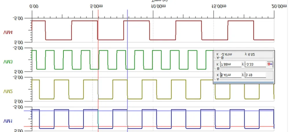
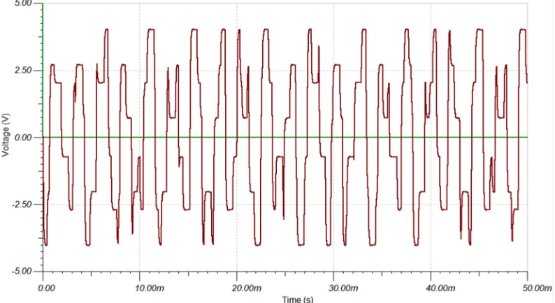
The input frequencies for each oscillator after the reservoir layer are measured before the parallel connection, as shown in Figure 4. The output coupling frequency is measured after the coupled oscillators achieve synchronization. Figure 5 and Figure 6 are the testing data from Figure 3 through Spice simulation with the same input frequencies (R =100 kΩ, R =500 kΩ, R =100 kΩ, R =300 kΩ) and different coupling weights (coupling resistance). The coupled oscillators synchronize in Figure 5 but fail to synchronize in Figure 6.
Figure 2. The output of the coupled Schmitt trigger based oscillatory neural network under real-time information. The coupled oscillators are synchronized completely. R1, R2, R3, R4 are the Resistors from Figure 3, R1 = 1 kΩ, R2= 1 kΩ, R3= 100 kΩ, R4= 100 kΩ.
From the simulation result, we find that the smaller the coupling resistance value, the stronger the coupling strength. On the contrary, the larger the coupling resistance value, the weaker the coupling strength. When the coupling resistance value of one oscillator is under a very small value (< 10 kΩ), and it is much smaller than the other oscillators, we define that oscillator with stronger coupling weight as
leader oscillator. In this paper, we choose the fixed R1 = R2
= 1 kΩ R3 = R4 = 100 kΩ. R1 and R2 are the two leaders, and
R3 and R4 are the two followers. The simulation result tells
us that when OSC1 and OSC2 work as leader oscillator, the
ONN almost always achieve synchronization and the synchronization frequency is close to the average value of the leader oscillators.
Figure 3. The output of the coupled Schmitt trigger based oscillatory neural network under real-time information. The coupled oscillators are not synchronized. R1, R2, R3, R4 are the Resistors from Figure 3. R1 = 100 kΩ, R2= 200 kΩ, R3= 300 kΩ, R4= 500 kΩ.
4.2. Weight Training
When we are ready to train weight to make predictions, we take the input signal and the output signal as our original data.
The more training data we use, the more accurate we get for a longer period. And then we compare the original data in the prediction.
following equation for MATLAB simulation: ∑& ! ! "# $!%"#
%'# sin +#, sin 3 +#. sin 5 (2)
Where ω=2πf.
4.2.1. Weight Training Method
The weight training matrix is shown as,
0
# # ! # , # #
# ! ! ! , ! !
…
# 2 ! 2 , 2 2
3 0 4# 4! … 42
3 + 0 5# 5! … 52
3 0 6# 6! … 62
3 (3)
Where f (t) is the first three harmonics of the Fourier series of each Schmitt trigger oscillator. w1,...,wn are the training weights,
b1,..., bn are the thresholds, which are unknown getting from the
training process, and y is the first three harmonics of the Fourier series of the synchronized frequency tested from the corresponding input.
We now show an example of how we can use the measured data from Spice simulation to train the weight. We start with the one-step learning performance of a 4-oscillator network. In our analysis, we use the following procedures.
1. Measure each oscillator's frequency before coupling and the frequency at the central bus after synchronization from Spice simulation.
2. Export the frequency data to Excel and transfer the data from Excel to MATLAB workspace, then compute the first three harmonic frequency for each oscillator and coupled oscillators in MATLAB. Data should be transposed as columns to be rows.
3. We are using the MATLAB Neural Network Toolbox to train the weight. Define the input as the first three harmonic frequency of each oscillator before coupling, the target as the first three harmonic frequency after synchronization. From the network type, we can choose the desired network type. In this example, we choose feed-forward with backpropagation. Select the training function as trainlm, adaption learning function as learngdm, and performance function as MSE (Mean Squared Error). 4. Repeat the previous step to find the best fitting. The weight
matrix can be read from MATLAB after fitting.
5. During the hardware simulation, we keep the coupling strength unchanged. We repeat step 1 by changing the R-value, as shown in Figure 3 in Spice. In a real experiment, R-value can be affected by the detected sensor value for pattern recognition in further study.
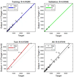
4.2.2. Performance of the Training
In our network, the input-output curve fitting with 70 percent of Training data, 15 percent of validation data, and 15 percent of testing data. Figure 7 shows the performance of neural network training regression. The role of nntool is to train the neural network and output the final network parameters: updated activations, errors, weights, and biases, (nn.a, nn.e, nn.W, nn.b) and training error: the sum squared error for each training mini-batch. Here, we perform a feed-forward backpropagation network. The more collected data from Spice simulation applying to the system, the better matching weights will be obtained, and more accuracy will be for the prediction.
4.3. Weight Retrieving
The simulation result above tells us that the regression process tries to predict a real number. While the training weight will vary every single time of the training. To improve the performance of the weight retrieving, and make simulation data better mapped to the hardware system, we use the classifier to predict a category to find the boundary of synchronization and non-synchronization. By defining the synchronization regions merging from the four coupled oscillators to varying frequencies of each oscillator to classify the status of synchronization and non-synchronization.
4.3.1. Dimensionality Reduction with PCA
In many fields of research and application, it is usually necessary to observe data containing multiple variables, collect large amounts of data, and analyze to find the law. Multi-variate big data sets will undoubtedly provide a wealth of information for research and application, but also increase the workload of data collection to some extent. More importantly, in many cases, there may be correlations between many variables, which increases the complexity of problem analysis. If each indicator is analyzed separately, the analysis is often isolated, and the information in the data cannot be fully utilized. Therefore, blindly reducing the indicator will lose a lot of useful information and lead to erroneous conclusions.
Therefore, it is necessary to find a reasonable method to reduce the loss of information contained in the original indicator while reducing the indicators that need to be analyzed, to achieve a comprehensive analysis of the collected data. Since there is a certain correlation between variables, it can be considered to change the closely related variables into as few new variables as possible, so that these new variables are irrelevant so that they can be represented by fewer comprehensive indicators. Various types of information that exist in each variable. PCA is a frequently used dimensionality reduction algorithm.
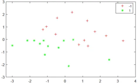
Figure 8. The mapping of the four oscillator frequencies in two dimensions. The green star represents the state in which the four oscillators are coupled and synchronized. The red cross represents the state in which the four oscillators are coupled and not synchronized.
In this sampled data set, we change the frequency of the oscillator by changing the resistance of each oscillator while keeping the value of the coupling weight un-changed. We collected twelve sets of oscillator frequencies that can be synchronized and twelve sets of oscillator frequencies that cannot be synchronized. Each set of data has four frequency values corresponding to four oscillators, meaning that we are collecting a set of four-dimensional data. After dimension reduction by PCA to a 2D plane, as shown in Figure 8.
4.3.2. Classification and Bound Search
To detect the boundary of the sampled data set after dimensionality reduction, we adopt an algorithm called Support Vector Machine (SVM), which was first proposed by Cortes and Vapnik in 1995 [30]. It shows many unique advantages in solving small sample, nonlinear, and high-dimensional pattern recognition and can be applied to function fitting and other machine learning problems.
The SVM method is based on the VC dimension theory and structural risk minimization principle of statistical learning theory. According to the limited sample information, we are seeking the best compromise between the complexity of the model (i.e., the accuracy of learning for specific training samples) and learning ability (i.e., the ability to identify any sample without error), to get the best promotion ability (or generalization ability). In general, if a linear function can separate the samples correctly, the data is said to be linearly separable. Otherwise, it is called the nonlinearly separable.
In this work, the synchronization regions emerging from a four-oscillator network response to the varying frequencies of each oscillator using SVM to classify. The reduced dimension data set can be considered as linear separable. After classification, the synchronization sample and non-synchronization sample are separated, as shown in Figure 9.
Figure 9. Two categories are being distinguished, and their samples are mapped in the two-dimensional plane. The middle line is a classification function that separates the two types of samples. The green star represents the state that the four coupled oscillators are synchronized. The red cross represents the state that the four coupled oscillators are not synchronized.
Expressed as
y wx + b (4) In which, w and b we can get from the MATLAB simulation. In this sample, the expression is
y ;0.5735x + 0.0677 (5)
4.3.3. Mapping the Boundary to the Hardware
The simulation result above gives us the boundary of synchronization and non-synchronization corresponding to = 100 kΩ, = 200 kΩ, = 300 kΩ, = 500 kΩ. When we train the classifier, we need to choose whether it is linear or nonlinear. The nonlinear problem needs to be mapped to the high-dimensional space to find the hyperplane. In this simulation, our sampled data is linearity separable, so we use linear classification and calculate the error. It also simplifies the calculation of the retrieval back to hardware. The following table summarizes the error of the linear classification of this work. As Table 1 shows, the sampled data are almost fit into the separation boundary.
Table 1. Nodes visited in boundary search.
Total nodes Synchronization nodes Non-synchronization nodes
Expected number 24 12 12
Separation number 24 11 11
Error 0 0.0833 0.0833
When given a set of non-synchronized data, by adjusting the slope and the bias of the separation line, which is also the w and b of a mathematical expression, we can fit it back to synchronize. Each slope and bias represents a set of coupling weights, which in the hardware is the coupling resistor. By simulating a couple of data and find the separation boundary, we can retrieve the separation boundary back to the hardware coupling resistance.
5. Discussion
Several data from hardware simulations are needed for training weights to get better performance with our system. We have demonstrated that a simple non-linear dynamical system--Schmitt trigger oscillatory neural network with simple external linear training weight can efficiently perform information processing in both hardware and software simulation. Therefore, as a result, our simple external scheme can replace the complex networks used in traditional Schmitt trigger based oscillatory neural networks. In comparison to mainstream digital computing paradigms, analog computing performs higher energy efficiency.
Besides, as far as we know, this experiment represents the hardware implementation of Schmitt trigger oscillatory neural network with results comparable to those obtained with linear regression using MATLAB Neural Network Toolbox. The sampled data includes four oscillators' frequencies, which represent a four-dimensional data set. The sampled data is linearity separable after using PCA to reduce the four-dimensional data set to the 2D plane. SVM is used to classify the synchronization and non- synchronization of sampled data. Retrieving the separation boundary back to the
hardware coupling resistance can be achieved by adjusting the slope and the bias of the separation line to match the coupling weight.
6. Conclusion
In this paper, a reservoir computing platform was studied to solve fitting problems in the non-linear complex dynamical system. Since the hysteresis of Schmitt trigger oscillator is challenging to model with conventional math model, instead of modeling the Schmitt trigger oscillator directly with math function, reservoir computing provides a solvable solution by keeping the existing non-linear complex dynamic connections and fitting the weight from outside between the reservoir layer and the output layer. In the process of training weights, we ignore the complicated relationships among the inputs generated by the harmonic outputs of the Schmitt trigger oscillators’ square wave signals. The advantage of training the weights externally is that we can use the existing system and substitute with another system that meets specific attributes. The training makes it possible for non-linear and high dimensional mapping substitutes with a simple linear algorithm. In this paper, we can predict the synchronization status of the unknown data set using SVM to find the boundary. Weight retrieving can be achieved by adjusting the slop and bias of the separation boundary.
Acknowledgements
National Science Foundation (NSF) Award ECCS-1813949 and Award CNS-1645863.
References
[1] Y. Li, Q. Ma, M. R. Haider, and Y. Massoud,”Ultra-low-power high sensitivity spike detectors based on modified nonlinear energy operator,” 2013 IEEE International Symposium on Circuits and Systems (ISCAS), Beijing, pp. 137-140, 2013. [2] A. K. M., Arifuzzman, M. S., Islam, and M. R. Haider.”A
Neuron Model-Based Ultralow Current Sensor System for Bioapplications.” Journal of Sensors, 2016.
[3] T., Zhang, M. R. Haider, Y. Massoud and J. Alexander.”An Oscillatory Neural Network Based Local Processing Unit for Pattern Recognition Applications.” Electronics, 8 (1), p. 64, 2019.
[4] Q. Ma, Y. Li, M. R. Haider and Y. Massoud,”A low-power neuromorphic bandpass filter for biosignal processing,” WAMICON 2013, Orlando, FL, 2013, pp. 1-3.
[5] Y. Li, Y. Massoud and M. R. Haider. Low-power high-sensitivity spike detectors for implantable VLSI neural recording microsystems. Analog Integrated Circuits and Signal Processing, 80 (3), pp. 449-457, 2014.
[6] I. E. Ebong, and P. Mazumder.”CMOS and memristor-based neural network design for position detection,” Proceedings of the IEEE, vol. 100, no. 6, pp. 2050–2060, 2011.
[7] A. U. Hassen and S. Anwar Khokhar,”Approximate in-Memory Computing on ReRAM Crossbars,” 2019 IEEE 62nd International Midwest Symposium on Circuits and Systems (MWSCAS), Dallas, TX, USA, pp. 1183-1186, 2019. [8] Y. Fang, C. N. Gnegy, T. Shibata, D. Dash, D. M. Chiarulli and
S. P. Levitan,”Non-Boolean Associative Processing: Circuits, System Architecture, and Algorithms,” in IEEE Journal on Exploratory Solid-State Computational Devices and Circuits, vol. 1, pp. 94-102, Dec. 2015.
[9] A. H. Kramer,”Array-based analog computation: principles, advantages and limitations.” In Proceedings of Fifth International Conference on Microelectronics for Neural Networks, pp. 68-79, 1996.
[10] L. Larger, M. C. Soriano, D. Brunner, L. Appeltant, J. M. Gutiérrez, L. Pesquera, C. R. Mirasso and I. Fischer,”Photonic information processing beyond Turing: an optoelectronic implementation of reservoir computing,” Optics express, vol. 20, no. 3, pp. 3241-3249, 2012.
[11] J. Li, Z. Qin, Y. Dai, F. Yin and K. Xu,”Real-time fourier transformation based on photonic reservior,” 2017 IEEE Photonics Conference (IPC), pp. 207-208, Orlando, FL, 2017. [12] J. Li, K. Bai, L. Liu and Y. Yi,”A deep learning based approach
for analog hardware implementation of delayed feedback reservoir computing system,” 2018 19th International Symposium on Quality Electronic Design (ISQED), pp. 308-313, Santa Clara, CA, 2018.
[13] L. Appeltant, M. C. Soriano, G. Van der Sande, J. Danckaert, S. Massar, J. Dambre, B. Schrauwen, C. R. Mirasso and I. Fischer,”Information processing using a single dynamical node as complex system,” Nature communications, no. 2, pp. 468, 2011.
[14] M. Freiberger, S. Sackesyn, C. Ma, A. Katumba, P. Bienstman and J. Dambre,”Improving Time Series Recognition and Prediction With Networks and Ensembles of Passive Photonic Reservoirs,” in IEEE Journal of Selected Topics in Quantum Electronics, vol. 26, no. 1, pp. 1-11, Art no. 7700611, Jan. -Feb. 2020.
[15] D. V. Buonomano and W. Maass,”State-dependent computations: Spatiotemporal processing in cortical networks,” Nature Reviews Neuroscience. vol. 10, no. 2, pp. 113–125, Feb. 2009.
[16] H. Jaeger and H. Haas,”Harnessing nonlinearity: predicting chaotic systems and saving energy in wireless communication,” Science, vol. 304, no. 5667, pp. 78–80, 2004.
[17] E. Vassilieva, G. Pinto, J. A. De Barros, and P. Suppes.”Learning pattern recognition through quasi-synchronization of phase oscillators,” IEEE Transactions on Neural Networks, vol. 22, no. 1, pp. 84-95, 2011.
[18] Z. Wang, H. He, G. P. Jiang, J. Cao,”Quasi-Synchronization in Heterogeneous Harmonic Oscillators with Continuous and Sampled Coupling,” IEEE Transactions on Systems, Man, and Cybernetics: Systems, Feb 22, 2019.
[19] D. A. Czaplewski, D. Antonio, J. R. Guest, D. Lopez, S. I. Arroyo and D. H. Zanette,”Enhanced synchronization range from non-linear micromechanical oscillators,” 2015 Transducers - 2015 18th International Conference on Solid-State Sensors, Actuators and Microsystems (TRANSDUCERS), pp. 2001-2004, Anchorage, AK, 2015. [20] J. Chen, J. Lu, X. Wu and W. X. Zheng,”Impulsive
synchronization on complex networks of nonlinear dynamical systems,” Proceedings of 2010 IEEE International Symposium on Circuits and Systems, Paris, pp. 421-424, 2010.
[21] H. Jaeger, and H. Haas,”Harnessing nonlinearity: predicting chaotic systems and saving energy in wireless communication,” Science no. 304, pp. 78–80, 2004.
[22] W. Maass, T. Natschläger, and H. Markram,”Real-time computing without stable states: a new framework for neural computation based on perturbations,” Neural Comput. no. 14, pp. 2531–2560, 2002.
[23] C. J. Commercon, and M. Guivarch.”Current transistor-transistor-inductor oscillator,” IEEE Proceedings-Circuits, Devices and Systems, vol. 141, no. 6, pp. 498-504, 1994.
[24] E. M. Izhikevich,”Polychronization: computation with spikes,” Neural computation, vol. 18, no. 2, pp. 245-282, Feb. 2006. [25] E. M. Izhikevich and Y. Kuramoto,”Weakly coupled
oscillators,” Encyclopedia of mathematical physics, New York: Elsevier, Jan. 2006.
[26] M. Itoh, and L. O. Chua,”Star cellular neural networks for associative and dynamic memories,” International Journal of Bifurcation and Chaos, vol. 14, no. 05, pp. 1725-1772, 2004. [27] F. C. Hoppensteadt, E. M. Izhikevich,”Oscillatory
neurocomputers with dynamic connectivity,” Phys. Rev. Lett, no. 82, pp. 2983–2986, 1999.
[29] Y. Fang.”Hierarchical associative memory based on oscillatory neural network.” PhD diss., University of Pittsburgh, 2013.