Volume-5 Issue-2
International Journal of Intellectual Advancements
and Research in Engineering Computations
Buffer dimensioning of dtn replication-based routing nodes with
hierarchical routing scheme
1
Mr. C.Mani M.C.A., M.Phil., M.E., Associate Professor,
2
Ms S.Kavitha Final MCA,
Departmet of MCA, Nandha Engineering College (Autonomous), Erode-52. E-Mail ID: [email protected], [email protected]
Abstract - Delay-Tolerant Networks (DTNs) operate in environments that are generally attributed by severe limitations such as intermittent connectivity. The DTN architecture handles such limitations with the help of store, carry, and forward paradigm, wherein the nodes physically carry the messages until they meet the destination. Underlying this paradigm is the node’s buffer space that becomes a costly real estate. Unless this buffer space is properly quantified, the routing performance would severely degrade.The DTN routing protocols that embody this paradigm would also resort to replication based strategies, in which multiple nodes carry the replica of the message. This is done in order to increase the delivery probability. Moreover, it inherently reduces the buffer loss at the source nodes when compared with the no relay nodes scenario. It would be interesting to investigate a way to quantify the buffer size and also perceive the reduction in buffer size of the source node with an increase in the number of relay nodes.
1. INTRODUCTION
DELAY-TOLERANT NETWORKS (DTNs) operate in environments that are generally attributed by severe limitations such as intermittent connectivity. The DTN architecture handles such limitations with the help of store, carry, and forward paradigm, wherein the nodes physically carry the messages until they meet the destination. Underlying this paradigm is the node’s buffer space that becomes a costly real estate. Unless this buffer space is properly quantified, the routing performance would severely degrade.
Furthermore, the DTN routing protocols that embody this paradigm would also resort to replication based strategies, in which multiple nodes carry the replica of the message. This is done in order to increase the delivery probability. Moreover, it inherently reduces the buffer loss at the source nodes when compared with the no relay nodes scenario. It would be interesting to investigate a way to quantify the buffer size and also perceive the reduction in buffer size of the
source node with an increase in the number of relay nodes. At this juncture, a systematic way of quantifying the buffer size is of utmost importance to tackle the buffer loss, in an efficient manner.
In the context of buffer space, much of the existing literature on DTN assumes either infinite buffer space or finite buffer space of the nodes in its system model. While there are a few works such as that study the average statistics of the node buffer, they are not helpful in bounding the buffer size. We were the first to address this problem in DTN and studied the buffer size in terms of the tail distribution of the overflow probability using Large Deviations Theory (LDT).
In, we focused on a single-hop forwarding problem in which every node directly transfers the messages to the corresponding destination nodes. This forwarding mechanism is also known as direct transmission protocol. Here, the service process of a source node is completely characterized by an exponential distribution involving the Inter-Meeting Time (IMT)–the time between the contacts–of the source node with the destination node. It is this service process abstraction that abstains from extending this framework to any multi-hop, replication-based DTN routing protocols.
In this letter, we therefore provide a radically different treatment to the bounding buffer problem, by using Markov modulated process and LDT. The capability of the proposed framework would render versatality in modeling a broad spectrum of multi-hop, replication-based routing protocols in the context of DTN.
2. A SIMPLIFIED DTN MODEL
We model the DTN as a graph where vertices are nodes and edges are sets of (representative) contacts. Our model allows only static nodes and nodes with strict repetitive motions [1]. A strict repetitive motion means that the node moves on a predetermined trajectory repetitively and the position of the node is a function of time in each repetition. Although this assumption might be quite strong in some situations, it is not unrealistic in many other cases since the motion of most real objects have repetitive patterns, and their positions at any particular time can be roughly estimated. Example networks to which such a model can be directly adopted are satellite networks where nodes have accurate periodic connectivity, and underwater acoustic networks where events that trigger the aberrancy of the nodes from their fixed trajectory are rare.
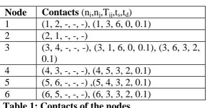
Figure 1: The simplified DTN model
Node Contacts (ni,nj,Tij,ts,td)
1 (1, 2, -, -, -), (1, 3, 6, 0, 0.1) 2 (2, 1, -, -, -)
3 (3, 4, -, -, -), (3, 1, 6, 0, 0.1), (3, 6, 3, 2, 0.1)
4 (4, 3, -, -, -), (4, 5, 3, 2, 0.1) 5 (5, 6, -, -, -) ,(5, 4, 3, 2, 0.1) 6 (6, 5, -, -, -), (6, 3, 3, 2, 0.1) Table 1: Contacts of the nodes
motions is a period of time such that, if n1,n2,...,nk
are at points p1,p2,...,pk respectively at any time t,
then they are at p1,p2,...,pk respectively at time t + k
× TS0. The relative motion cycle TS of a set S of
nodes (including static nodes and nodes with strict repetitive motions) is equal to TS0, if S0 ⊆ S (S0 =6 ∅), and S0 is the set of all mobile nodes in S.
For simplicity, TS of S = {ni,nj} is denoted by Tij. It
is obvious that if Ti and Tj are the motion cycles of
ni and nj respectively, then Tij equals the least
common multiple (LCM) of Ti and Tj. A similar
result holds when S has more than two elements.
Once the relative motion cycle Tij of nodes ni and nj
is known, the set of contacts C occurring within any period of time equal to Tij can be used to
represent all the other contacts [2]. In this paper, a predicted contact is represented by a tuple (ni,nj,Tij,tstart,tduration), and a persistent contact by
(ni,nj,−,−,−) where tstart and tduration are the starting
time and the duration (which depends on speed and transmission range) of the contact.
With the representative contacts for a set V of nodes in the network, one can use the optimal time-space Dijkstra’s algorithm, such as the ones in and to calculate the shortest path between a pair of nodes in V. Since our routing is unicast and there are usually multiple paths with the same minimal delay, we design an extended time-space Dijkstra’s algorithm which first finds all paths with the minimal delay and then chooses one among those paths with the least hop-count randomly [3]. This algorithm is used in DHR to route with local contact information in some levels of the hierarchical network. It is also used to compute the optimal routing solution on the global topology that is the basis upon which the routing performance of DHR is evaluated.
3. BUFFER DIMENSIONING FRAMEWORK FOR THE REPLICATION-BASED ROUTING PROTOCOL
In this section, we present the buffer dimensioning framework for the replication-based routing protocol. Here, the source node makes replica of the message to any relay node it meets. Based on the replication strategy adapted by the relay nodes, various routing protocols are conceived. Some of them are as follows: (i) when the relay nodes also replicate messages among themselves, then the corresponding protocol is called epidemic routing and (ii) when the relay nodes resort to direct transmission forwarding scheme, then the corresponding routing protocol is called two-hop routing protocol .
As in any replication based protocols, the routing process is followed by a recovery mechanism to wipeout the replicas of the just delivered message in the system. Without loss of generality, we consider a VACCINE recovery mechanism, in which the acknowledgement of the delivered message is spread to all the nodes in the network. This form of spreading is akin to the epidemic spreading that happens in a reverse direction [5]. Upon receipt of the acknowledgment the nodes either discard the delivered message or stay resistant from receiving it in the future. In other words, these nodes are said to be vaccinated or recovered. This process continues until all nodes are recovered in the system. However, we are interested in the recovery of the source node so that the delivered message is evicted.
Next we build the buffer dimensioning framework in an incremental fashion, starting from considering no-relay case and proceed towards extending it to the replication-based scenario involving relay nodes.
3.1 No Relay nodes
6 3 1
In this scenario, the source node needs to meet the destination node to offload the message. Under the given mobility model, the IMT of the source-destination node pairs are Independent and Identically Distributed (IID) with exponential distribution of parameter μ as defined[4]. Our objective is to find a bound on the buffer size of the source node. Under this setting, the incoming message sees an exponential time before leaving the queue. We abstract this to a queueing model with a constant service rate C. The parameters of this constant-service queue are defined as follows:
• The arrival process of the queue is Poisson with parameter λ.
• The incoming messages are assumed to bring a hypothetical work load which is exponentially distributed with parameter μ. And this hypothetical workload is due to the IMT of the node pairs.
3.2 With Relay Nodes
Here we extend the effective bandwidth approach discussed in the previous section, by incorporating the multi-copy replication-based routing enabled by the relay nodes.
The source node creates a replica of the incoming message to any non-destination nodes it meets. This happens at the rate of Nμ. And invariant to any routing protocol’s replication strategy (such as epidemic routing and two-hop routing), the worst-case rate at which the recovery process kick-starts would be Nμ2, after which 2 recovered nodes (the deliverer and the destination) are created. Let X(t)t≥0 denote the environment process
representing the manifestation of the recovery process to evict the message at the source node [2]. And this process evolves as a Continuous-Time Markov Chain (CTMC). While state 1 is represented by the source node with the message to be delivered, the remaining states represent the number of recovered nodes in the system. The service process of the source node is therefore modulated by this CTMC.
4. MULTILEVEL CLUSTERING AND HIERARCHICAL ROUTING
This section reviews a multilevel clustering and hierarchical routing algorithm in static networks on which our proposed algorithm is based. Organizing a network into a hierarchical structure could make the management of routing tables scalable. Clustering offers such a structure, and it suits networks with relatively large numbers of nodes [3]. Multilevel clustering, which is clustering applied recursively over clusterheads, is feasible and effective in large networks.
4.1 Multilevel clustering
Clustering is conducted first by electing clusterheads. Then, non-clusterheads choose clusters to join and become members. There are two kinds of clustering algorithms. One is the cluster algorithm. In this algorithm, a node selects itself as a clusterhead if it has the highest priority among its unclustered neighbors. A non-clusterhead joins the cluster of a non-clusterhead that has the highest priority among the node’s neighboring clusterheads.
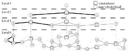
Figure 2: Lowest ID hierarchical clustering.
The other is the core algorithm in which each node selects a node in its neighborhood including itself with the highest priority as a clusterhead and then joins that node’s cluster. The main difference between these two are whether clusterheads could be neighbors [4]. Also, the cluster algorithm runs sequential rounds while the core algorithm needs one round to complete. In our work, we use the cluster algorithm. There are many ways to define node priorities. The lowest ID algorithm is widely used. In the lowest ID cluster algorithm, the lower a node’s ID, the higher is its priority[4]. The hierarchical network as the result of the multilevel clustering using the lowest ID algorithm on the physical network shown in level 0 of the hierarchy.
The hierarchical network is a logical tree of nodes in a homogeneous network, where nodes and links above level 0 in the hierarchy are conceptual. A node in level k+1 corresponds to a cluster (or a clusterhead) in level k, and the ID of the level k + 1 node is the same as that of the clusterhead in the level k cluster. We use subscripts to denote the level to which a node belongs. We use 61 to denote that the node with
label 6 is in level 1, which represents the cluster in level 0 consisting of 60, 80 and 240. A hierarchy
address of a node is a sequence of IDs of the clusters of the node and its clusters in all levels. For instance, the hierarchy address of the physical node 8 is (13,22,61,80), where 61 is the
cluster of 80 in level 1, 22 is the cluster of 61 (and
thus of 80) in level 2, and 13 the cluster in level 3.
link between any two nodes of two clusters on level k, then there is a link between the nodes representing these clusters in level k + 1. For instance, there is a link between 61 and 21 since
there is a link between 60 and 130. We call 60 a
gateway and 130 a remote gateway from cluster 61
to cluster 21. Each level k + 1 link is associated
with a delay which is equal to the delay of the shortest path between the corresponding level k clusterheads [1]. For instance, if the delay of the link between 60 and 130 is 3 and that of the link
between 130 and 20 is 2, then the delay of the link
between 61 and 21 is 5, since 5 is the delay of the
shortest path (the only path in this example) between 60 and 20.
4.2 Hierarchical routing
Hierarchical routing facilitates the hierarchical network as a topology abstraction and may not generate a shortest path. The advantage of hierarchical routing is that it is scalable (logarithmic) for localized traffic patterns, and it does not need location information.
Hierarchical routing requires that the source has the hierarchy address of the destination. If only the ID of the destination is available, the source can resort to using location service. Hierarchical routing is a hop-by-hop routing rather than a source routing. Before any routing, each node in the network needs to obtain the topology information of its clusters in all levels. For instance, node 8 has the topology information consisting of all the thick links [2]. Note that it includes the gateway links, such as links (60,130) and (21,41). The availability of this
routing algorithm releases the clusterheads burden of relaying every message forwarded to other clusters.
Each node makes its forwarding decision via the following steps: find the lowest level k where the source s and the destination d have a common cluster, define the intermediate source s0 and the intermediate destination d0, which are the level k clusters of s and d respectively, use the optimal time-space Dijkstra’s algorithm to find the next hop n0 on the shortest path from s0 to d0 based on the level k topology information of s. if k = 0, n0 is the forwarding decision of s, otherwise go back to step 3 with a new k = k −1, a new d0
being the remote gateway from s0 to n0, and a new s0 being the the node on level k (new k) which is either s or a cluster of s.
5. MULTILEVEL CLUSTERING AND HIERARCHICAL ROUTING IN DTNS The information in a level k+1 link in a static hierarchical network contains a time-invariant delay which is simply the sum of the delays of the level k links on a shortest path between the level k
clusterheads. The challenge in multilevel clustering in our DTN model is that the delay information in the links is time-variant. A method needs to be proposed to aggregate the time-varying information to the links in the hierarchical network from . their immediately lower level.
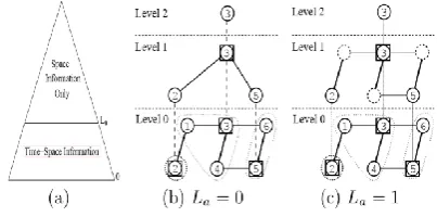
Figure 3: A hierarchical network with aggregated contact information given an aggregation level
5.1 Multilevel clustering in DTNs
Each node on level 0 of the hierarchical network corresponds to a physical node, and there is a link between two level 0 nodes if there are contacts between their physical nodes. To allow the links in each level in the hierarchical network to have time-variant delay information, we store in each link a set of contacts. Contacts are stored in the 5-element tuple format presented [4]. A level 0 link stores all contacts between the two end nodes. A level k+1 link aggregates all contacts in the level k links that form paths between the corresponding level k clusterheads, which includes those between clusterheads and gateways and those between gateways.
The size of the aggregated contact information in the links increases exponentially as their level increases. To ensure scalability, the aggregation should stop at a certain level which we call the aggregation level La. The links above level La
maintain time-invariant delays just as in the static hierarchical network.
The delay on the links above level La is calculated
in the same way as in the static hierarchial network. To calculate the time-invariant delay on level La + 1, each link on level La also needs to
have a time-invariant delay. We use the weighted average delay which is the expectation (in statistics) of the time-variant delays of the shortest paths between these two end nodes of the level La link. In our DTN model, the weighted
average delay can be calculated with the set of shortest paths within a period of time equal to the LCM of the cycles of the contacts stored in the link.
We use two methods to compress the aggregated contact information. The first method, which has already been presented, compresses the space information by removing the time-dimension information in the links above level La. Analytical study and simulation in later
sections show that its impact on the routing performance is slight when La is not very small.
An intelligent improvement is to decide (a) Level 0 average delay whether to compress according to the volume of the contact information and the variance (in statistic) of the timevariant delays of the link.
The second compression method, which removes contacts from the links, is implemented as follows. Suppose (u,v) is a level k link, T is the LCM of the motion cycles of the contacts stored by (u,v), {ti} is
the set of time slots which is a partition of T such that within each ti the set of shortest paths between
u and v does not change, and {Sij} is the set of
contacts on the jth shortest path during ti. A boolean
function E is constructed in the following steps. First, construct terms Eij with the names of all
contacts in {Sij} as literals [3]. Second, construct
disjunctive normal forms (a disjunction of terms) Ei
with all Eijs. Finally, construct E which is a
conjunction of all Eis. Here, a set of contacts
satisfies Ei if they form a shortest path during ti, and
a set R of contacts satisfying E can be used to calculate the delay of the shortest paths between u and v at any time. This compression algorithm reduces the size of R to reduce the storage and communication overhead while retains most of the important contacts for the links.
Again, an intelligent improvement is to choose the smallest set of contacts whose shortest paths’ variance from the actual shortest paths is below a particular threshold. It should be able to further reduce the size of contact information when, for instance, 20% of the contacts form 80% of the shortest paths.
Our proposed DTN Hierarchical Routing (DHR) is quite straightforward after the hierarchical network has been built. DHR is also a hop-by-hop routing. Each node makes its forwarding decision in two phases. The first phase runs only when the highest level Lc, on which the cluster of the current node
and that of the destination are different, is greater than L a. In this phase, the static hierarchical
routing, as presented [2], runs on the levels (from Lc to La +1) where delay on the links are
time-invariant. The result of this phase is an intermediate destination d0 of level La.
When Lc ≤ La, the first phase does not run, and d0 is
set to the clusterhead of the destination in level Lc.
The second phase, which we called aggregation routing, has the following steps: (1) all contact
information in the links from level 0 to level La that
are stored by the current node are aggregated to form a graph G. That is, G includes all contacts in the links in the clusters of the current node from level 0 to level La in the hierarchical network. (2)
the optimal time-space Dijkstra’s algorithm is performed on G to find a shortest path p from the current node to d0. The first hop on p is the current node’s forwarding decision.
6. ANALYSIS
6.1 Routing performance
In this subsection, we will analyze the possible impact of removing the time dimension at higher levels (above La). We estimate the inaccuracy of
using the weighted average delay to represent the delay of a time variant link with the relative deviation , where µn is the expectation of the
delay of a n-hop link (i.e., the weighted average delay) and σn is the standard deviation of the delays
of the shortest paths.
7. RELATED WORKS
Jain, Fall, and Patra exhaustively formulated the DTN routing problem under different degrees of knowledge about the network. Specifically, the Dijkstra’s algorithm is used to calculate the shortest path with contacts being predictable, and also a linear programming approach which calculates the optimal routes across the network with additional knowledge of the global traffic demand. Merugu, Ammar, and Zegura proposed a time-space routing algorithm that is similar in spirit to the Dijkstra’s algorithm [1].
Among the approaches in deterministic routing exploited deterministic trajectory of mobile nodes to help deliver data, improve data delivery performance, and reduce energy consumption in nodes. Wu, Yang, and Dai used semi-deterministic trajectory of mobile node to achieve deterministic results of several routing schemes. However, such a trajectory is selected from a set of predefined hierarchical structured routes.
Much work has been done on multilevel clustering and hierarchical routing in MANETs. In the multilevel clustering approaches such as DART, L+, MMWN, and WHIRL , certain nodes are elected as clusterheads. These clusterheads in turn select higher level clusterheads, up to some desired level. A node’s address is defined as a sequence of clusterhead identifiers, one per level, allowing the size of routing tables to be logarithmic in the size of the network. One problem with explicit clusterheads is that routing through clusterheads creates traffic bottlenecks. In L+, this issue is partially solved by allowing nearby nodes to route packets instead of the clusterhead.
8. CONCLUSION
In this paper, we have proposed DTN Hierarchical Routing (DHR) in a simplified DTN model where nodes have strict repetitive motions. We constructed a hierarchical network which provides a compressed time-space topology abstraction of the network in our DTN model. Two aggregated contact information compression algorithms are presented for better scalability. Simulation results showed that the performance of DHR approximates that of the optimal time space Dijkstra’s algorithm in terms of delay and hop-count in networks of different ratio of mobile and static nodes. Simulation results are consistent with theoretical analysis in that the performance of DHR increases as the sourcedestination distance increases, and the routing performance degrades slightly as more contact information in the hierarchical network is compressed.
Our future work will focus on improving the contact information compression algorithms. Two of such improvements have been suggested in Section 4.2. Relaxing the constraints in our DTN model and making necessary changes to the hierarchical clustering and routing algorithms are also very important future work to increase the applicability of DHR to more general DTN models.
REFERENCES
[1] B. Chen and R. Morris. L+: Scalable landmark routing
and address lookup fo multi-hop wireless network. In MIT LCS Technical Report 837, March 2002.
[2] J. Haas, J. Y. Halpern, and L. Li. Gossip-based ad hoc
routing. In Proc. of IEEE INFOCOM, 2002.
[3] S. Jain, K. Fall, and R. Patra. Routing in a delay tolerant
network. In Proc. of ACM SIGCOMM, 2004.
[4] A. Lindgren, A. Doria, and O. Schelen. Probabilistic
routing in intermittently connected networks. Lecture Notes in Computer Science, 3126:239–254, Aug 2004.
[5] G. Pei, M. Gerla, X. Hong, and C. Chiang. A wireless