Determining the best population-level alcohol consumption model and its impact on estimates of alcohol-attributable harms

(1)

R E S E A R C H

Open Access

Determining the best population-level alcohol

consumption model and its impact on estimates

of alcohol-attributable harms

Tara Kehoe

1,2*

, Gerrit Gmel

1

, Kevin D Shield

1,9

, Gerhard Gmel

1,4,5,6

and Jürgen Rehm

1,3,7,8,9

Abstract

Background:

The goals of our study are to determine the most appropriate model for alcohol consumption as an

exposure for burden of disease, to analyze the effect of the chosen alcohol consumption distribution on the

estimation of the alcohol Population- Attributable Fractions (PAFs), and to characterize the chosen alcohol

consumption distribution by exploring if there is a global relationship within the distribution.

Methods:

To identify the best model, the Log-Normal, Gamma, and Weibull prevalence distributions were

examined using data from 41 surveys from Gender, Alcohol and Culture: An International Study (GENACIS) and

from the European Comparative Alcohol Study. To assess the effect of these distributions on the estimated alcohol

PAFs, we calculated the alcohol PAF for diabetes, breast cancer, and pancreatitis using the three above-named

distributions and using the more traditional approach based on categories. The relationship between the mean

and the standard deviation from the Gamma distribution was estimated using data from 851 datasets for 66

countries from GENACIS and from the STEPwise approach to Surveillance from the World Health Organization.

Results:

The Log-Normal distribution provided a poor fit for the survey data, with Gamma and Weibull

distributions providing better fits. Additionally, our analyses showed that there were no marked differences for the

alcohol PAF estimates based on the Gamma or Weibull distributions compared to PAFs based on categorical

alcohol consumption estimates. The standard deviation of the alcohol distribution was highly dependent on the

mean, with a unit increase in alcohol consumption associated with a unit increase in the mean of 1.258 (95% CI:

1.223 to 1.293) (R

2

= 0.9207) for women and 1.171 (95% CI: 1.144 to 1.197) (R

2

= 0. 9474) for men.

Conclusions:

Although the Gamma distribution and the Weibull distribution provided similar results, the Gamma

distribution is recommended to model alcohol consumption from population surveys due to its fit, flexibility, and

the ease with which it can be modified. The results showed that a large degree of variance of the standard

deviation of the alcohol consumption Gamma distribution was explained by the mean alcohol consumption,

allowing for alcohol consumption to be modeled through a Gamma distribution using only average consumption.

Keywords:

Alcohol consumption, Empirical distribution, Gamma distribution, Log-Normal distribution, Weibull

dis-tribution, Population-Attributable Fraction, Exposure disdis-tribution, Up-estimation, Per capita consumption, Mean,

Standard deviation

Introduction

Alcohol consumption is a component cause [1] for over

200 International Classification of Diseases (ICD-10)

three-digit codes [2,3]. In other words, a fraction, usually

called the Population-Attributable Fraction (PAF) of the

incidence of these diseases, would disappear if exposure

to one of the causal components was eliminated [4-7]

(in the case of alcohol, under the counterfactual

sce-nario of every person being a lifetime abstainer). The

proportion of the diseases caused by alcohol

consump-tion in a component cause model for a populaconsump-tion is

determined by both the patterns and volume of alcohol

consumption and by the relative risks associated with

* Correspondence: [email protected]

1_{Centre for Addiction and Mental Health (CAMH), Toronto, Canada}

Full list of author information is available at the end of the article

(2)

each exposure level [3,8]. For most major diseases where

alcohol plays a role (for example, alcohol-attributable

cancers, pancreatitis, and cirrhosis of the liver), the

aver-age volume of alcohol consumption alone was found to

be an adequate predictor of the risk [3,8-10]; however,

some diseases and injuries (for example, ischemic heart

disease, unintentional injuries, and intentional injuries)

were found to be also dependent on drinking patterns

[11-14].

The calculation of an alcohol PAF involves a

three-stage process: 1) estimation of an exposure distribution

of alcohol, 2) establishment of the relative risk function,

and 3) the solving of the equation for the PAF [15].

Since the distribution of alcohol consumption on an

international level has not been agreed upon, the

com-mon approach is to estimate the PAF using categorical

measurements rather than modeling it in a more

mathe-matically appropriate continuous manner [16,17]. The

mathematical expression is as follows:(Formula 1)

PAF

=

k

i=1

P

i

(

RR

i

−

1)

k

i=1

P

i

(

RR

i

−

1) + 1

where

i

is the exposure category with baseline

expo-sure or no expoexpo-sure,

i = 0, RR

i

is the relative risk at

exposure level

i

compared to no consumption, and

P

i

is

the prevalence of the

j

th

category of exposure.

When a continuous distribution for the volume of

alcohol consumption is used, this calculation can be

represented by the following formula:(Formula 2)

PAF

(

x

) =

P

a

RR

a

+

P

ex

RR

ex

+

150

0

P

(

x

)

RR

(

x

)

dx

- 1

P

a

RR

a

+

P

ex

RR

ex

+

150

0

P

(

x

)

RR

(

x

)

dx

where

P

_a

is the prevalence of lifetime abstainers,

RR

_a

is the relative risk of lifetime abstainers,

P

_ex

is the

preva-lence of former drinkers,

RR

_ex

is the relative risk of

for-mer drinkers,

x

is the average volume of alcohol

consumption per day,

P(x)

is the prevalence of alcohol

consumption, and

RR(x)

is the relative risk of drinkers

[15]. Although this is the most accurate way to calculate

a PAF, it requires that the distribution of alcohol

con-sumption be known. Previous attempts at modeling

alcohol consumption using a Log-Normal distribution

have been criticized for various reasons [18,19];

how-ever, the Log-Normal distribution has provided adequate

approximations for most applications [20,21]. Recently,

more adaptable distributions such as the Gamma

distri-bution have been favored over the Log-Normal

distribu-tion [15,22], and it has been suggested that a mixing of

distributions is needed to separately model the

fre-quency of drinking and the quantity of alcohol

con-sumed [23].

There are two main instruments to monitor alcohol

exposure currently used by countries and international

organizations: 1) general population surveys and 2)

esti-mates of per capita consumption, where per capita

con-sumption is an aggregate measure of recorded,

unrecorded, and tourist per capita consumption of

alco-hol (derived from sales, production, and other economic

statistics) [9,24,25]. These instruments, however, have

limitations [26].

There are no available surveys for many countries, and

in some cases where they do exist they do not allow for

the accurate estimation of the volume of consumption,

as these surveys only ask about the absence or presence

of drinking [27]. Existing surveys often considerably

underestimate real consumption levels [28-30] by

typi-cally covering only 30% to 60% of alcohol sales [26]. As

a result, per capita consumption figures are considered

to be a best estimate of overall volume of consumption

in a country [31]; however, per capita consumption does

not provide any disaggregated statistic and, thus, does

not provide age- and gender-specific consumption

esti-mates. Since in some instances the risk relationship

between alcohol consumption and disease-specific

mor-tality is dependent on gender as well as on age, alcohol

exposure by gender and age is required to estimate the

PAF and to calculate the alcohol-attributable burden of

disease in a population [3].

The problems noted above with respect to surveys

lead to an underestimated burden of disease attributable

to alcohol consumption when PAFs are calculated from

population data without adjustment. As a consequence,

methods have been developed to triangulate both

aver-age alcohol consumption derived from population

sur-veys and from per capita consumption information

[15,26]. However, current PAF calculation methods are

based on categorical estimates of consumption with

alcohol consumption being corrected by multiplying the

two top alcohol consumption categories by the inverse

of the estimated undercoverage (per capita

consump-tion/the estimated per capita consumption from the

sur-vey) [17]. For most categories of disease where there is

an association with volume of alcohol consumption, the

dose-response relationship is nonlinear and, thus,

distri-bution estimates of alcohol consumption by age and

gender are required for accurate estimates of alcohol

PAFs [3].

(3)

distribution of alcohol consumption that can easily be

modeled to make the fit more compatible with per

capita consumption data and that also has properties

that make it possible to estimate the exposure

distribu-tion for countries that lack survey data except for

esti-mates of prevalence of abstention. Thus, the first aim of

this study is to assess internationally if alcohol

consis-tently follows one of the three well-known right-skewed

distributions, Log-Normal, Gamma, or Weibull, and to

determine if the chosen exposure distribution has a

sig-nificant effect on the estimation of a PAF, using the

PAFs for pancreatitis, diabetes, and breast cancer as

examples. The second aim of this study is to investigate

if a global relationship between parameters exists so that

a distribution of alcohol consumption can be estimated

based on mean alcohol consumption.

Methods

Description of underlying surveys

This study used data from Gender, Alcohol and Culture:

An International Study (GENACIS), from the European

Comparative Alcohol Study (ECAS), and from the

STEPwise approach to Surveillance (STEPS). Survey

data were collected for the average volume of

consump-tion for Argentina, Australia (two surveys from Australia

were used: Australia and Australia1), Austria, Belize,

Brazil, Canada, Costa Rica, Czech Republic, Denmark,

Finland, France, Germany, Hungary, Iceland, India,

Ire-land, Isle of Man, Israel, Italy, Japan, Kazakhstan,

Mex-ico, Netherlands, Nicaragua, Nigeria, Norway, Peru,

Spain, Sri Lanka, Sweden, Switzerland, Uganda, United

Kingdom, Uruguay, and the United States of America

from GENACIS (three surveys from the United States of

America were used: USA1, USA2, and USA3; USA1 was

a 2001 longitudinal study that surveyed women only,

and USA2 and USA3 were 1995-1996 and 2000

National Alcohol Surveys, respectively); for Finland,

France, Germany, Italy, Sweden, and the United

King-dom from ECAS; and for Cameroon, Côte D

’

Ivoire,

Dominica, Democratic Republic of the Congo, Eritrea,

Kuwait, Mali, Mozambique, American Samoa, Barbados,

Benin, Botswana, Cape Verde, Republic of the Congo,

Cook Islands, Indonesia, Madagascar, St. Kitts and

Nevis, Swaziland, Zambia, Fiji, Kiribati, Marshall Islands,

Mongolia, Nauru, Solomon Islands, Tokelau, Tonga,

Vanuatu, Micronesia, and Samoa from STEPS. (For

information on sampling methodology and the questions

used in GENACIS surveys see [33-35], ECAS see [30],

and STEPS see [36]). For most of the GENACIS surveys

and for the ECAS surveys alcohol consumption was

measured by a beverage-specific usual

quantity-fre-quency technique (i.e., asking separate questions on

usual frequency of drinking, and then eliciting the usual

quantity per drinking occasion), and in the remaining

GENACIS surveys alcohol consumption was measured

by a global quantity-frequency measure. In the STEPS

surveys alcohol consumption was measured in standard

drinks consumed in the seven days preceding the survey.

All data from surveys were divided by sex and age into

eight age groups; 15-24, 25-34, 35-44, 45-54, 55-64,

65-74, 75-84, and 85 +.

Methods for fitting the distributions

As alcohol consumption distributions have been shown

to have a unimodal shape, [19,37,38] we evaluated the

fit of the Log-Normal, Gamma, and Weibull

distribu-tions (unimodal distribudistribu-tions commonly used to fit

right-skewed empirical data) to determine the most

appropriate distribution to model alcohol consumption

from national survey data. The Log-Normal, Gamma,

and Weibull probability densities are similar in shape,

but have significantly different tail behaviors. In the

past, alcohol consumption has been more commonly

modeled by the Log-Normal distribution as it is used to

model continuous random quantities that are

right-skewed and is based on the normal distribution, making

it easy to fit, test, and modify [20,21]. Although alcohol

consumption is frequently modeled using the

Log-Nor-mal distribution, empirical distributions often deviate

considerably from the Log-Normal model. In

compari-son, the Gamma and Weibull distributions have a scale

parameter and a shape parameter, making them more

adaptable since the scale parameter can stretch or

com-press the distribution.

The Log-Normal distribution is a function of the

mean (

μ

) and standard deviation (

s

) parameters, and

describes a random variable x where log (x) is normally

distributed. The probability density function of the

Log-Normal distribution can be expressed as follows:

f

(

x

;

μ

,

σ

) =

1

x

σ

√

2

π

exp

−

(log

x

−

μ

)

2

σ

2

where x > 0 and -

∞

<

μ

<

∞

,

s

> 0 The Gamma

dis-tribution is characterized by a shape (

) and a scale

parameter (

θ

), has a mean of

θ

and a standard

devia-tion of

√

κθ

2

.

The probability density function of the

Gamma distribution can be expressed as follows:

f

(

x

;

κ

,

θ

) =

x

κ−1

θ

κ

(

κ

)

exp

−

x

θ

where

x

>

0,

>

0,

θ

>

0

and

(

κ

) =

∞

0

t

κ−1

exp

{−t}

dt

Similar to the Gamma

distri-bution, the Weibull distribution is commonly

(4)

Weibull distribution has a mean of

θ

1

γ

+ 1

and a

standard deviation of

θ

2

γ

+ 1

−

1

γ

+ 1

2

,

where

(

x

)

=

∞

0

t

x−1

exp

{−

t

}

dt

is the Gamma function

evaluated at

x

. The probability density function of the

Weibull distribution is expressed as follows:

f

(

x

;

θ

,

γ

) =

γ

θ

x

θ

γ−1

exp

−

x

θ

γ

where x

≥

0,

g

> 0,

θ

> 0 Maximum likelihood

estima-tion was used to fit all three distribuestima-tion models to the

drinking population data obtained from GENACIS and

ECAS. All missing values were excluded from the fitted

models. The Newton-Raphson algorithm was used to

optimize the likelihood equations solving for the

maxi-mum likelihood estimates of the unknown parameters

[39]. Data values of alcohol consumption over 300 g/day

were truncated to 300 g/day. Numerical integration

uti-lizing the trapezoidal rule was used to characterize each

distribution.

Method for deriving the alcohol PAF

We performed a sensitivity analysis where the alcohol

PAFs for pancreatitis, diabetes, and breast cancer were

calculated using a continuous model (Log-Normal,

Gamma, and Weibull) and using a categorical model in

order to see if the chosen exposure distribution had an

effect on the estimation of the alcohol PAF. All PAFs

were calculated with zero alcohol consumption as the

counterfactual scenario, similarly to the Comparative

Risk Analysis for alcohol. This counterfactual scenario

under certain circumstances of a light drinking average

alcohol consumption without heavy drinking occasions

may not reflect the theoretical minimum risk depending

on the distribution of diseases and cause of death in a

society. However, for this paper these considerations are

not relevant. The relative risks of lifetime abstainers and

former drinkers for pancreatitis, diabetes, and breast

cancer were obtained from the meta-analysis [40-42].

In order to illustrate that the alcohol PAF estimates

based on the Gamma distribution model deviated only

slightly from the PAF derived from the categorical

model, we calculated the difference between the PAFs

calculated for both models.

Methods for characterizing the gamma distributions

The Gamma distribution can be characterized by a

shape () and a scale parameter (θ), where the mean

and the standard deviation of the Gamma distribution

can be obtained directly from the parameter estimates

as follows:

μ

=

κθ

and

σ

=

√

κθ

2

Since the mean of the Gamma distribution is equal to

the mean of the empirical distribution, the mean of the

Gamma distribution does not need to be estimated from

the shape and scale parameters.

A maximum likelihood algorithm (see description

above) was used to obtain the shape and scale

para-meters using the maximum likelihood function for the

shape and scale parameters of the Gamma distribution:

l(κ,θ) = (κ−1)

N

i=1 ln(xi)−

N

i=1

xi

θ −N·κ·ln(θ)−N·ln((κ))

Regression analysis

The maximum likelihood method was used to fit a

Gamma model in order to summarize the alcohol

con-sumption of 66 countries by gender and age (in total 851

datasets [422 for women; 429 for men]). After the data

was fit by a Gamma model, the relationship between the

Gamma mean and the Gamma standard deviation was

examined using various general linear models. The

per-formance of the general linear models was then assessed

by how well the assumption of homoscedasticity was

upheld and based on the distribution of the residuals.

All data analyses were performed in R version 2.13.0

[43].

Results

Modeling alcohol consumption as a distribution

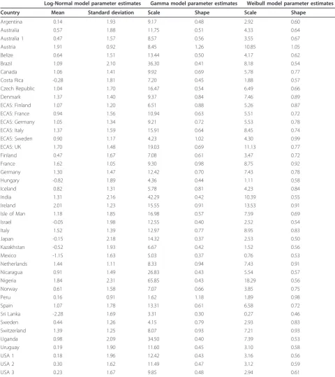
The three distributions, Log-Normal, Gamma, and

Wei-bull, were fit to 41 datasets; parameter estimates are

outlined in Table 1 for women and in Table 2 for men.

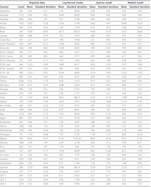
The mean and standard deviation estimates from the

empirical data and the estimates from each fitted model

are summarized in Table 3 for women and in Table 4

for men. When comparing the empirical mean to each

distribution

’

s mean, we observed that the mean

esti-mates from the Weibull distribution were much closer

to the empirical mean than were the Log-Normal

distri-bution mean estimates, while the mean estimates from

the Gamma distribution were equal to the empirical

mean. When comparing the standard deviation

esti-mates, the estimates from the Log-Normal distribution

deviated furthest from the empirical data, while there

was no statistically significant difference between the

empirical standard deviation estimate and the standard

deviation estimates from either of the Weibull or the

Gamma distributions.

(5)

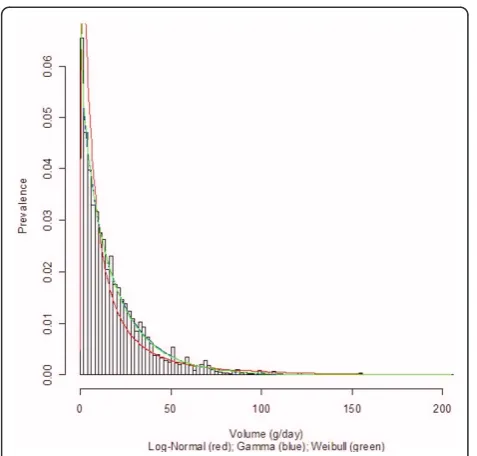
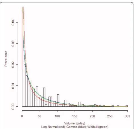
Uganda, were selected to display their density curves

(Log-Normal, Gamma, and Weibull) superimposed on

the population-based data histograms; see Figures 1, 2,

3, 4, 5, and 6 for both women and men. We observed a

common trend among men in Figures 2, 4, and 6: the

Log-Normal distribution tended to underestimate the

number of men who drank 25 g/day to 50 g/day,

whereas the Gamma and Weibull distributions

accu-rately estimated alcohol consumption for these

popula-tions. A similar trend was observed with respect to

Table 1 Parameter estimates from Log-Normal, Gamma, and Weibull models for women from 43 datasets

Log-Normal model parameter estimates Gamma model parameter estimates Weibull model parameter estimates

Country Mean Standard deviation Scale Shape Scale Shape

Argentina 0.14 1.93 9.17 0.48 2.92 0.60

Australia 0.57 1.88 11.75 0.51 4.33 0.64

Australia 1 0.47 1.57 8.57 0.56 3.55 0.67

Austria 1.91 0.92 8.45 1.26 10.85 1.05

Belize 0.64 1.51 13.44 0.50 4.17 0.62

Brazil 1.09 2.10 36.30 0.41 8.18 0.54

Canada 1.06 1.41 9.92 0.69 5.78 0.77

Costa Rica -0.28 1.81 7.20 0.45 1.88 0.57

Czech Republic 1.04 1.70 16.47 0.54 6.49 0.66

Denmark 1.37 1.40 9.37 0.84 7.46 0.89

ECAS: Finland 1.07 1.20 6.51 0.88 5.26 0.87

ECAS: France 0.94 1.56 10.94 0.63 5.51 0.72

ECAS: Germany 1.05 1.34 9.21 0.72 5.53 0.78

ECAS: Italy 1.37 1.59 15.91 0.64 8.45 0.74

ECAS: Sweden 0.90 1.17 4.23 1.02 4.30 0.99

ECAS: UK 1.70 1.48 19.03 0.69 11.13 0.77

Finland 0.47 1.67 7.08 0.61 3.47 0.72

France 1.62 1.05 9.30 0.98 8.75 0.92

Germany 1.30 1.47 12.42 0.70 7.43 0.78

Hungary -0.82 1.89 4.36 0.44 1.11 0.58

Iceland 0.82 1.31 5.78 0.81 4.23 0.84

India 1.31 2.16 42.29 0.42 10.39 0.55

Ireland 2.01 1.23 15.55 0.91 13.53 0.91

Isle of Man 1.18 1.85 16.98 0.57 7.59 0.69

Israel -0.05 1.98 12.55 0.40 2.52 0.54

Italy 1.52 1.39 12.97 0.77 8.95 0.83

Japan -0.15 2.18 14.32 0.37 2.53 0.50

Kazakhstan -0.52 1.93 6.67 0.42 1.52 0.56

Mexico -1.15 1.63 5.03 0.37 0.76 0.53

Netherlands 1.44 1.11 8.33 0.94 7.43 0.91

Nicaragua 0.91 1.49 26.83 0.43 5.54 0.57

Nigeria 1.84 2.31 65.85 0.43 18.29 0.56

Norway 0.61 1.58 7.07 0.66 3.85 0.75

Peru 0.16 0.91 1.62 1.18 1.89 0.98

Spain 1.07 1.78 13.31 0.61 6.58 0.72

Sri Lanka -2.28 1.69 3.31 0.30 0.27 0.46

Sweden 0.44 1.26 4.15 0.79 2.93 0.83

Switzerland 1.39 1.25 8.07 0.93 7.21 0.93

Uganda 0.98 2.09 34.50 0.40 7.39 0.53

Uruguay 0.19 1.90 11.60 0.45 3.10 0.58

USA 1 0.18 1.96 12.42 0.43 3.16 0.56

USA 2 0.30 1.62 11.49 0.47 3.12 0.59

(6)

women from Germany and Uganda who drank between

10 g/day to 30 g/day and for Sri Lankan women who

drank between 0.5 g/day to 2.0 g/day.

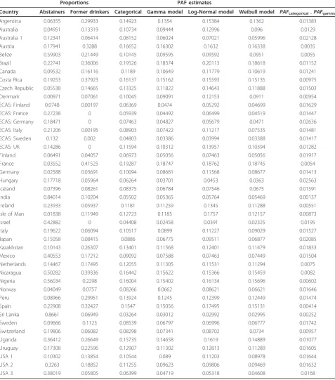
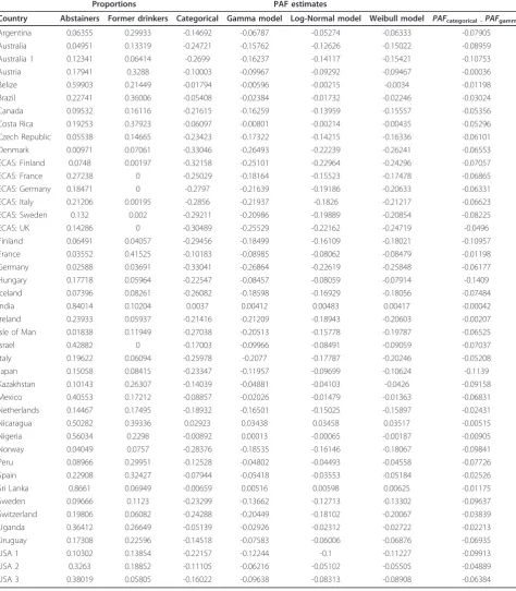
Alcohol PAF estimates modeled using the

Log-Nor-mal, Gamma, and Weibull distributions, together with

the proportion estimates for lifetime abstainers and

for-mer drinkers, are listed in Table 5 for breast cancer

(women), Tables 6 and 7 for diabetes (women and men,

respectively), and Tables 8 and 9 for pancreatitis

(women and men, respectively).

The alcohol PAF estimates that incorporated the

Gamma and Weibull distributions are very similar and,

for the most part, are within 1% of one another. Since

the Log-Normal distribution is known to have a heavy

tail, and this study includes data values for alcohol

con-sumption up to 300 g/day, the alcohol PAF estimates

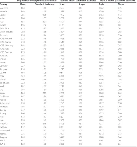
Table 2 Parameter estimates from Log-Normal, Gamma, and Weibull models for men from 41 datasets

Log-Normal model parameter estimates Gamma model parameter estimates Weibull model parameter estimates

Country Mean Standard deviation Scale Shape Scale Shape

Argentina 1.84 1.68 25.33 0.64 13.62 0.75

Australia 1.63 1.69 18.79 0.67 10.99 0.78

Austria 2.85 0.96 19.72 1.33 27.52 1.13

Belize 2.06 1.55 37.69 0.59 16.85 0.69

Brazil 1.57 2.01 47.07 0.44 12.55 0.57

Canada 1.96 1.42 21.64 0.74 14.04 0.81

Costa Rica 1.13 1.87 23.50 0.49 7.71 0.61

Czech Republic 2.58 1.55 38.84 0.75 26.59 0.83

Denmark 2.28 1.24 18.05 0.98 17.33 0.96

ECAS: Finland 2.22 1.18 16.68 0.99 16.13 0.95

ECAS: France 2.18 1.48 26.19 0.75 17.56 0.82

ECAS: Germany 1.92 1.33 16.43 0.84 12.84 0.87

ECAS: Italy 2.22 1.40 20.68 0.87 17.43 0.92

ECAS: Sweden 1.79 1.26 13.48 0.87 10.94 0.88

ECAS: UK 2.85 1.30 38.19 0.88 31.78 0.90

Finland 1.76 1.51 17.08 0.75 11.58 0.83

France 2.44 1.25 25.29 0.88 21.08 0.90

Germany 2.27 1.37 21.29 0.88 18.07 0.92

Hungary 1.10 1.81 17.13 0.55 6.95 0.67

Iceland 1.64 1.25 9.84 0.96 9.17 0.95

India 2.24 1.95 69.20 0.49 23.75 0.62

Ireland 3.04 1.18 38.57 0.98 36.94 0.95

Isle of Man 2.22 1.78 39.38 0.63 20.51 0.74

Israel 1.02 1.87 22.11 0.48 6.85 0.61

Italy 2.44 1.30 21.80 0.96 20.92 0.99

Japan 1.63 2.19 37.45 0.49 13.60 0.63

Kazakhstan 1.87 1.76 36.80 0.55 14.69 0.67

Mexico 1.34 1.90 33.23 0.46 9.68 0.59

Netherlands 2.28 1.17 17.45 1.00 17.27 0.98

Nicaragua 2.03 1.52 38.43 0.58 16.28 0.68

Nigeria 2.47 1.78 55.90 0.60 26.97 0.71

Norway 1.66 1.44 15.92 0.74 10.25 0.80

Peru 1.13 1.17 8.89 0.76 5.60 0.79

Spain 2.28 1.49 25.30 0.81 19.04 0.87

Sri Lanka 1.30 2.18 57.93 0.37 10.71 0.51

Sweden 1.12 1.32 8.20 0.79 5.83 0.83

Switzerland 2.37 1.12 17.65 1.05 18.27 0.97

Uganda 2.75 1.79 70.07 0.61 35.42 0.73

Uruguay 1.69 1.84 34.78 0.52 12.88 0.64

USA 2 1.41 1.72 25.65 0.53 9.50 0.64

(7)

Table 3 Mean and standard deviation estimates from the empirical data, Log-Normal model, Gamma model, and the

Weibull model for alcohol consumption of women from 43 datasets

Empirical data Log-Normal model Gamma model Weibull model

Country Count Mean Standard deviation Mean Standard deviation Mean Standard deviation Mean Standard deviation

Argentina 381 4.38 6.77 7.35 46.50 4.38 6.34 4.39 7.69

Australia 1172 6.04 9.52 10.40 60.39 6.04 8.42 6.06 9.90

Australia 1 3002 4.84 7.81 5.47 17.86 4.84 6.44 4.69 7.22

Austria 1916 10.62 13.26 10.36 11.94 10.62 9.47 10.66 10.20

Belize 386 6.74 16.63 5.92 17.44 6.74 9.52 5.98 10.02

Brazil 283 14.80 29.63 26.75 240.21 14.80 23.18 14.27 28.60

Canada 5850 6.88 10.79 7.82 19.76 6.88 8.26 6.75 8.90

Costa Rica 367 3.21 6.33 3.90 19.86 3.21 4.81 3.00 5.57

Czech Republic 1023 8.97 15.12 12.08 50.02 8.97 12.16 8.74 13.71

Denmark 1042 7.89 8.85 10.48 26.03 7.89 8.59 7.89 8.85

ECAS: Finland 469 5.71 9.65 6.00 10.77 5.71 6.09 5.63 6.47

ECAS: France 382 6.85 9.83 8.64 27.71 6.85 8.66 6.77 9.54

ECAS: Germany 512 6.93 21.77 7.05 15.85 6.62 7.80 6.39 8.30

ECAS: Italy 404 10.23 14.99 14.08 48.17 10.23 12.76 10.17 13.94

ECAS: Sweden 433 4.32 4.58 4.87 8.35 4.32 4.28 4.32 4.36

ECAS: UK 498 13.14 19.31 16.34 46.06 13.14 15.81 12.97 17.02

Finland 882 4.35 7.83 6.45 25.27 4.35 5.55 4.28 6.07

France 4206 9.14 11.79 8.78 12.42 9.14 9.22 9.08 9.83

Germany 4164 8.72 12.97 10.88 30.24 8.72 10.41 8.60 11.17

Hungary 883 1.92 5.31 2.62 15.31 1.92 2.90 1.75 3.22

Iceland 1072 4.70 7.41 5.34 11.37 4.70 5.21 4.63 5.53

India 85 17.67 26.94 38.01 388.74 17.67 27.33 17.88 35.44

Ireland 378 14.20 17.69 16.05 30.35 14.20 14.86 14.14 15.54

Isle of Man 469 9.67 13.20 17.91 97.33 9.67 12.81 9.77 14.57

Israel 1938 4.98 12.52 6.70 46.91 4.98 7.91 4.46 9.04

Italy 1219 9.93 11.72 11.91 28.76 9.93 11.35 9.90 12.01

Japan 864 5.27 11.72 9.17 97.39 5.27 8.68 5.02 11.15

Kazakhstan 401 2.80 7.91 3.78 23.87 2.80 4.32 2.50 4.78

Mexico 1406 1.88 7.32 1.20 4.39 1.88 3.07 1.37 2.82

Netherlands 1505 7.84 10.50 7.83 12.20 7.84 8.08 7.78 8.58

Nicaragua 147 11.43 34.88 7.52 21.56 11.43 17.51 8.94 16.78

Nigeria 200 28.45 41.91 91.55 1322.58 28.45 43.28 30.12 57.50

Norway 1004 4.64 7.03 6.39 21.38 4.64 5.73 4.59 6.21

Peru 620 1.91 3.07 1.78 2.03 1.91 1.76 1.90 1.95

Spain 427 8.07 11.17 14.34 69.00 8.07 10.36 8.12 11.50

Sri Lanka 38 1.00 2.93 0.42 1.70 1.00 1.82 0.64 1.63

Sweden 2226 3.29 4.51 3.42 6.75 3.29 3.69 3.24 3.94

Switzerland 5362 7.50 10.07 8.77 17.04 7.50 7.78 7.48 8.09

Uganda 280 13.78 26.60 23.46 206.14 13.78 21.80 13.25 27.17

Uruguay 375 5.17 12.02 7.35 43.87 5.17 7.75 4.91 9.05

USA 1 854 5.37 10.39 8.11 54.33 5.37 8.17 5.21 9.95

USA 2 1310 5.35 14.44 5.00 17.90 5.35 7.84 4.76 8.46

(8)

from the Log-Normal distribution tend to be much

lar-ger and unrealistic when compared to the estimates

from the Gamma and Weibull distributions.

Overall, the PAF estimates from the categorical model,

Gamma model, and Weibull model are relatively similar

when the survey data are more compact, but for those

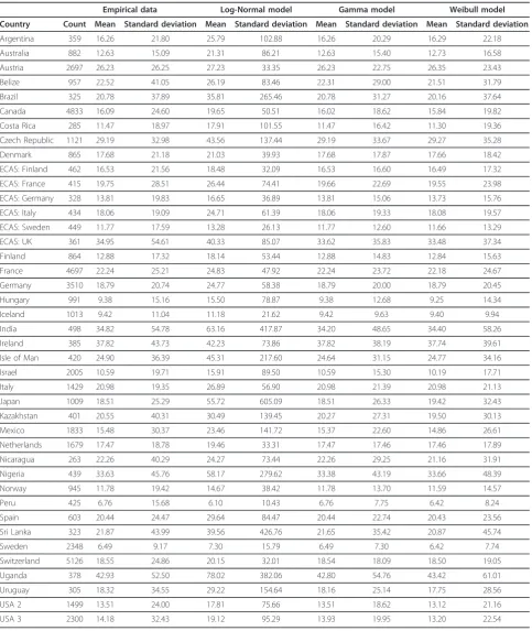
Table 4 Mean and standard deviation estimates from the empirical data, Log-Normal model, Gamma model, and the

Weibull model for alcohol consumption of men from 41 datasets

Empirical data Log-Normal model Gamma model Weibull model

Country Count Mean Standard deviation Mean Standard deviation Mean Standard deviation Mean Standard deviation

Argentina 359 16.26 21.80 25.79 102.88 16.26 20.29 16.29 22.18

Australia 882 12.63 15.09 21.31 86.21 12.63 15.40 12.73 16.58

Austria 2697 26.23 26.25 27.23 33.35 26.23 22.75 26.35 23.43

Belize 957 22.52 41.05 26.19 83.46 22.31 29.00 21.51 31.79

Brazil 325 20.78 37.89 35.81 265.46 20.78 31.27 20.16 37.64

Canada 4833 16.09 24.60 19.65 50.51 16.02 18.62 15.84 19.82

Costa Rica 285 11.47 18.97 17.91 101.55 11.47 16.42 11.30 19.36

Czech Republic 1121 29.19 32.98 43.56 137.44 29.19 33.67 29.27 35.28

Denmark 865 17.68 21.18 21.03 39.93 17.68 17.87 17.66 18.42

ECAS: Finland 462 16.53 21.56 18.48 32.09 16.53 16.60 16.49 17.32

ECAS: France 415 19.75 28.51 26.44 74.41 19.66 22.69 19.55 23.98

ECAS: Germany 328 13.81 19.83 16.65 36.89 13.81 15.06 13.73 15.76

ECAS: Italy 434 18.06 19.09 24.71 61.39 18.06 19.33 18.08 19.57

ECAS: Sweden 449 11.77 17.59 13.28 26.13 11.77 12.60 11.66 13.29

ECAS: UK 361 34.95 54.61 40.33 85.07 33.62 35.83 33.48 37.34

Finland 864 12.88 17.32 18.14 53.44 12.88 14.83 12.84 15.63

France 4697 22.24 25.21 24.83 47.92 22.24 23.72 22.18 24.67

Germany 3510 18.79 20.74 24.77 58.38 18.79 20.00 18.79 20.45

Hungary 991 9.38 15.16 15.50 78.87 9.38 12.68 9.25 14.34

Iceland 1013 9.42 11.04 11.18 21.62 9.42 9.63 9.40 9.94

India 498 34.82 54.78 63.16 417.87 34.20 48.65 34.40 58.26

Ireland 385 37.82 43.73 42.23 73.86 37.82 38.19 37.74 39.61

Isle of Man 420 24.90 36.39 45.31 217.60 24.64 31.15 24.77 34.16

Israel 2005 10.59 19.71 15.91 89.50 10.59 15.30 10.19 17.71

Italy 1429 20.98 19.35 26.89 56.90 20.98 21.39 20.98 21.13

Japan 1009 18.51 25.29 55.72 605.09 18.51 26.33 19.42 32.43

Kazakhstan 401 20.55 40.31 30.49 139.45 20.27 27.31 19.50 30.13

Mexico 1833 15.48 30.37 23.46 141.72 15.37 22.60 14.86 26.61

Netherlands 1679 17.47 18.78 19.46 33.31 17.47 17.46 17.46 17.89

Nicaragua 263 22.26 40.29 24.27 73.44 22.26 29.25 21.16 31.91

Nigeria 439 33.63 45.76 58.17 279.62 33.38 43.19 33.66 48.39

Norway 945 11.78 19.42 14.67 38.42 11.78 13.70 11.59 14.57

Peru 425 6.76 15.68 6.10 10.43 6.76 7.75 6.42 8.24

Spain 603 20.44 24.47 29.64 84.47 20.44 22.74 20.43 23.56

Sri Lanka 323 21.87 43.99 39.56 426.76 21.65 35.42 20.87 45.74

Sweden 2348 6.49 9.17 7.30 15.79 6.49 7.30 6.42 7.74

Switzerland 5126 18.55 24.86 20.15 32.01 18.54 18.09 18.50 19.05

Uganda 378 42.93 52.50 78.02 382.06 42.80 54.76 43.42 61.01

Uruguay 305 18.32 34.55 29.22 154.64 18.16 25.14 17.75 28.56

USA 2 1499 13.51 24.00 17.81 75.66 13.51 18.62 13.12 21.16

(9)

countries where data are more spread out, PAF

esti-mates are more susceptible to sampling bias for diseases

with a relatively linear or exponential risk relationship

with alcohol, such as pancreatitis and breast cancer. For

example, for Brazilian men the alcohol consumption

prevalence data tend to be very spread out when

com-pared to men from France, leading to a small difference

in the PAFs for pancreatitis. However, this trend does

not apply when we look at a disease, such as diabetes,

that has a J-shaped relative risk function. If we look at

the same example, we find that the alcohol PAFs for

dia-betes provide similar estimates from the categorical

model, Gamma model, Log-Normal model, and Weibull

model for men from both Brazil and France. This is due

to the fact that the relative risk functions are exponential

Figure 1Alcohol consumption distribution in grams per day of

pure alcohol for women in Germany. Alcohol consumption distribution in grams per day of pure alcohol for women in Germany.

Figure 2Alcohol consumption distribution in grams per day of pure alcohol for men in Germany.

Figure 3Alcohol consumption distribution in grams per day of pure alcohol for women in Sri Lanka.

(10)

for pancreatitis and are J-shaped for diabetes and thus

have different properties. The J-shaped curve in some

cases leads to a negative PAF (which represents the

frac-tion of deaths prevented) as the risk of diabetes at the

population level is less under current levels of alcohol

consumption than under the counterfactual scenario of

no alcohol consumption.

Characterizing the alcohol consumption gamma

distribution

Based on data from GENACIS and STEPS, the mean

daily average per capita alcohol consumption among

drinkers was estimated to be 7.549 grams for women

(the Gamma standard deviation was 9.862) and 18.292

grams for men (the Gamma standard deviation was

22.015) (see Table 10).

After analyzing the association between the Gamma

mean and the Gamma standard deviation, a strong

lin-ear relationship was established. Analysis of the

resi-duals of various general linear models led to the

conclusion that a general linear model with a normal

distribution and an identity link (i.e., a linear regression

model) is the best possible model to characterize the

relationship between the standard deviation of the

Gamma distribution and the mean of the Gamma

dis-tribution. As a statistical interaction was determined to

be present by gender for the relationship between the

Gamma mean and the Gamma standard deviation, this

linear relationship was modeled separately for men and

for women.

Figures 7 and 8 illustrate the linear fit for women

and men, respectively. The linear regressions indicate

that a unit increase in mean alcohol consumption is

associated with an increase of 1.258 (95% CI: 1.223 to

1.293) in the standard deviation of the Gamma alcohol

consumption distribution for women and 1.171 (95%

CI: 1.144 to 1.197) in the standard deviation of the

Gamma alcohol consumption distribution for men.

Additionally, for women the linear regression indicated

that 92.07% of the variation of the standard deviation

of the Gamma distribution was explained by the mean,

while for men 94.74% of the variation of the standard

deviation of the Gamma distribution was explained by

the mean.

Regression diagnostics indicated that there were some

outliers. For women, two data points from Nigeria and

one from Uganda were identified as influential

observa-tions, while for men, two observations in Germany and

one in Nigeria were identified as influential observations.

There was no indication of a lack of homoscedasticity

for any of the regression models (Additional file 1).

Discussion

Both the Gamma and the Weibull distributions

sum-marized the population distribution of average volume

of alcohol consumption more accurately than did the

Log-Normal distribution. Moreover, for the Gamma and

Weibull distributions the ratio of mean to standard

deviation was comparable across all countries,

irrespec-tive of drinking patterns and the survey measure used to

measure alcohol consumption. Overall, both the Gamma

and Weibull distributions yield similar PAFs and could

Figure 5Alcohol consumption distribution in grams per day of

pure alcohol for women in Uganda.

(11)

be used in descriptive alcohol epidemiology. Although

not examined specifically, these outcomes would also

apply to PAFs that are calculated when using a

counter-factual scenario where alcohol consumption is decreased

due to a policy or intervention such as taxation. Since

the Weibull distribution is a more complicated

distribu-tion and less flexible than the Gamma distribudistribu-tion, and

since it is possible to shift the Gamma distribution

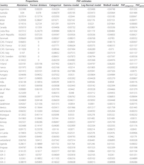
Table 5 Proportion estimates for lifetime abstainers and former drinkers, as well as Population-Attributable Fraction

(PAF) estimates for breast cancer using a categorical model and continuous models (Gamma, Log-Normal, and

Weibull) for women

Proportions PAF estimates

Country Abstainers Former drinkers Categorical Gamma model Log-Normal model Weibull model PAFcategorical -PAFgamma

Argentina 0.06355 0.29933 0.14923 0.1354 0.15384 0.1362 0.01383

Australia 0.04951 0.13319 0.10734 0.09444 0.12996 0.096 0.0129

Australia 1 0.12341 0.06414 0.08152 0.06024 0.07021 0.05996 0.02128

Austria 0.17941 0.3288 0.16652 0.16302 0.1632 0.16338 0.0035

Belize 0.59903 0.21449 0.10145 0.09595 0.09592 0.0951 0.0055

Brazil 0.22741 0.36006 0.19526 0.18374 0.20113 0.18618 0.01152

Canada 0.09532 0.16116 0.1189 0.10649 0.11779 0.10619 0.01241

Costa Rica 0.19253 0.37923 0.16137 0.15162 0.15593 0.15135 0.00975

Czech Republic 0.05538 0.14665 0.13325 0.11822 0.14643 0.11888 0.01503

Denmark 0.00971 0.07061 0.10045 0.09091 0.12153 0.0911 0.00954

ECAS: Finland 0.0748 0.00197 0.06369 0.0474 0.05292 0.04699 0.01629

ECAS: France 0.27238 0 0.05939 0.04492 0.06499 0.04519 0.01447

ECAS: Germany 0.18471 0 0.07463 0.04827 0.05679 0.0471 0.02636

ECAS: Italy 0.21206 0.00195 0.08903 0.07422 0.11217 0.07535 0.01481

ECAS: Sweden 0.132 0.002 0.04803 0.03386 0.03994 0.03388 0.01417

ECAS: UK 0.14286 0 0.11594 0.10312 0.13957 0.10394 0.01282

Finland 0.06491 0.04057 0.06973 0.05056 0.07463 0.05056 0.01917

France 0.03552 0.41525 0.19287 0.18747 0.18762 0.18745 0.0054

Germany 0.02588 0.03691 0.10094 0.08681 0.11568 0.08677 0.01413

Hungary 0.17718 0.05964 0.06264 0.03701 0.0453 0.0363 0.02563

Iceland 0.07396 0.08261 0.08375 0.06784 0.07546 0.0675 0.01591

India 0.84014 0.10204 0.05502 0.05365 0.05764 0.05469 0.00137

Ireland 0.23933 0.05937 0.1181 0.11259 0.1345 0.11288 0.00551

Isle of Man 0.01838 0.11949 0.12723 0.1185 0.1757 0.12157 0.00873

Israel 0.42882 0 0.04408 0.02458 0.0391 0.02325 0.0195

Italy 0.19622 0.06094 0.10517 0.0899 0.11227 0.09029 0.01527

Japan 0.15058 0.08415 0.0886 0.06775 0.09511 0.06877 0.02085

Kazakhstan 0.10143 0.26307 0.13401 0.11568 0.12401 0.11479 0.01833

Mexico 0.40553 0.17212 0.09092 0.07588 0.07463 0.07449 0.01504

Netherlands 0.14467 0.17495 0.12055 0.11305 0.11531 0.11294 0.0075

Nicaragua 0.50282 0.39336 0.16442 0.15622 0.15366 0.15459 0.0082

Nigeria 0.56034 0.2298 0.16004 0.15402 0.16134 0.15696 0.00602

Norway 0.04049 0.0757 0.08266 0.0662 0.08621 0.06621 0.01646

Peru 0.08966 0.29951 0.13924 0.1245 0.12399 0.12449 0.01474

Spain 0.22908 0.32427 0.1547 0.15056 0.17495 0.15131 0.00414

Sri Lanka 0.8661 0.06949 0.03264 0.03012 0.02992 0.02995 0.00252

Sweden 0.09666 0.1123 0.08539 0.06797 0.06996 0.06777 0.01742

Switzerland 0.19806 0.06082 0.08298 0.07341 0.08702 0.0734 0.00957

Uganda 0.36412 0.26649 0.15735 0.14658 0.1619 0.14889 0.01077

Uruguay 0.17308 0.22596 0.12907 0.11302 0.12813 0.11289 0.01605

USA 1 0.10302 0.13854 0.10544 0.089 0.11203 0.08978 0.01644

USA 2 0.3263 0.18852 0.11255 0.09623 0.09806 0.09469 0.01632

(12)

upwards (necessary in modeling the burden of disease

attributable to alcohol consumption), the Gamma

distri-bution is the best distridistri-bution for modeling alcohol

consumption.

Modeling survey alcohol consumption data alone

with-out correcting the distribution for undercoverage will

lead to inaccurate alcohol PAFs as self-reported survey

data typically underestimate alcohol consumption based

(PAF) estimates for diabetes using a categorical model and continuous models (Gamma, Log-Normal, and Weibull) for

women

Argentina 0.06355 0.29933 -0.14692 -0.06787 -0.05274 -0.06333 -0.07905

Australia 0.04951 0.13319 -0.24721 -0.15762 -0.12626 -0.15022 -0.08959

Australia 1 0.12341 0.06414 -0.2699 -0.16237 -0.14117 -0.15421 -0.10753

Austria 0.17941 0.3288 -0.10003 -0.09967 -0.09292 -0.09467 -0.00036

Belize 0.59903 0.21449 -0.01794 -0.00596 -0.00215 -0.0034 -0.01198

Brazil 0.22741 0.36006 -0.05408 -0.02384 -0.01732 -0.02246 -0.03024

Canada 0.09532 0.16116 -0.21615 -0.16259 -0.13959 -0.15557 -0.05356

Costa Rica 0.19253 0.37923 -0.06097 -0.00801 -0.00214 -0.00435 -0.05296 Czech Republic 0.05538 0.14665 -0.23423 -0.17322 -0.14215 -0.16336 -0.06101

Denmark 0.00971 0.07061 -0.33046 -0.26493 -0.22239 -0.26241 -0.06553

ECAS: Finland 0.0748 0.00197 -0.32158 -0.25101 -0.22964 -0.24296 -0.07057

ECAS: France 0.27238 0 -0.25029 -0.18164 -0.15523 -0.17478 -0.06865

ECAS: Germany 0.18471 0 -0.2797 -0.21639 -0.19186 -0.20633 -0.06331

ECAS: Italy 0.21206 0.00195 -0.2856 -0.21937 -0.1826 -0.21217 -0.06623

ECAS: Sweden 0.132 0.002 -0.29211 -0.20986 -0.19889 -0.20854 -0.08225

ECAS: UK 0.14286 0 -0.30489 -0.25529 -0.22162 -0.24719 -0.0496

Finland 0.06491 0.04057 -0.29456 -0.18499 -0.16109 -0.18021 -0.10957

France 0.03552 0.41525 -0.10183 -0.08985 -0.08062 -0.08479 -0.01198

Germany 0.02588 0.03691 -0.33041 -0.26864 -0.22619 -0.25848 -0.06177

Hungary 0.17718 0.05964 -0.22547 -0.08457 -0.08059 -0.07914 -0.1409

Iceland 0.07396 0.08261 -0.26082 -0.18598 -0.16929 -0.18056 -0.07484

India 0.84014 0.10204 0.0037 0.00412 0.00483 0.00417 -0.00042

Ireland 0.23933 0.05937 -0.21416 -0.21209 -0.18943 -0.20603 -0.00207

Isle of Man 0.01838 0.11949 -0.27038 -0.20513 -0.15778 -0.19787 -0.06525

Israel 0.42882 0 -0.17003 -0.09966 -0.08491 -0.09059 -0.07037

Italy 0.19622 0.06094 -0.25978 -0.2077 -0.17787 -0.20246 -0.05208

Japan 0.15058 0.08415 -0.23347 -0.11957 -0.09699 -0.10624 -0.1139

Kazakhstan 0.10143 0.26307 -0.14039 -0.04881 -0.04103 -0.0426 -0.09158

Mexico 0.40553 0.17212 -0.08857 -0.02026 -0.01479 -0.01363 -0.06831

Netherlands 0.14467 0.17495 -0.18932 -0.16501 -0.15025 -0.15897 -0.02431

Nicaragua 0.50282 0.39336 0.02923 0.03438 0.03458 0.03517 -0.00515

Nigeria 0.56034 0.2298 -0.00892 0.00013 -0.00065 -0.00187 -0.00905

Norway 0.04049 0.0757 -0.28376 -0.18535 -0.16146 -0.18067 -0.09841

Peru 0.08966 0.29951 -0.12528 -0.04802 -0.04493 -0.04558 -0.07726

Spain 0.22908 0.32427 -0.07944 -0.05418 -0.03553 -0.05184 -0.02526

Sri Lanka 0.8661 0.06949 -0.00659 0.00516 0.00598 0.00625 -0.01175

Sweden 0.09666 0.1123 -0.23299 -0.13662 -0.12713 -0.13302 -0.09637

Switzerland 0.19806 0.06082 -0.24288 -0.20449 -0.18102 -0.20067 -0.03839

Uganda 0.36412 0.26649 -0.05139 -0.02926 -0.02312 -0.02722 -0.02213

Uruguay 0.17308 0.22596 -0.14518 -0.07583 -0.06006 -0.06876 -0.06935

USA 1 0.10302 0.13854 -0.22157 -0.12244 -0.1 -0.11227 -0.09913

USA 2 0.3263 0.18852 -0.11105 -0.06216 -0.05102 -0.05505 -0.04889

(13)

on sales or taxation (e.g., [26]). In other words, alcohol

surveys often do not accurately represent the population

due to undercoverage where some members of the

popu-lation are inadequately represented (or excluded) or due

to response bias [30]. Accordingly, a method must be

developed that will shift the exposure distribution so that

it is consistent with per capita consumption data in order

to correct for survey bias and allow for a more accurate

(PAF) estimates for diabetes using a categorical model and continuous models (Gamma, Log-Normal, and Weibull) for

men

Argentina 0.02488 0.08209 -0.06204 -0.04912 -0.03488 -0.04748 -0.01292

Australia 0.04 0.078 -0.06679 -0.05195 -0.03473 -0.05064 -0.01484

Austria 0.07014 0.15774 -0.03393 -0.0344 -0.03358 -0.03185 0.00047

Belize 0.20958 0.28647 0.01671 0.02142 0.02176 0.02153 -0.00471

Brazil 0.14516 0.2724 0.01291 0.01974 0.0221 0.01964 -0.00683

Canada 0.05019 0.1359 -0.04406 -0.03732 -0.02801 -0.03536 -0.00674

Costa Rica 0.07212 0.24279 -0.00984 0.00218 0.01119 0.00484 -0.01202

Czech Republic 0.02653 0.07235 -0.04347 -0.03926 -0.03536 -0.04003 -0.00421

Denmark 0.00669 0.02899 -0.08567 -0.08015 -0.06768 -0.0783 -0.00552

ECAS: Finland 0.06855 0 -0.08737 -0.0843 -0.07434 -0.08173 -0.00307

ECAS: France 0.12632 0 -0.07771 -0.06634 -0.05575 -0.06515 -0.01137

ECAS: Germany 0.11828 0 -0.08546 -0.07494 -0.06289 -0.073 -0.01052

ECAS: Italy 0.107 0 -0.08652 -0.07515 -0.06007 -0.07519 -0.01137

ECAS: Sweden 0.07803 0 -0.08431 -0.07873 -0.06794 -0.07597 -0.00558

ECAS: UK 0.10422 0 -0.06259 -0.04982 -0.05368 -0.04976 -0.01277

Finland 0.03181 0.05196 -0.07492 -0.06375 -0.04797 -0.06205 -0.01117

France 0.01975 0.2008 -0.02168 -0.0214 -0.01805 -0.02032 -0.00028

Germany 0.01415 0.03101 -0.08136 -0.07386 -0.05941 -0.07326 -0.0075

Hungary 0.04696 0.04052 -0.07032 -0.0531 -0.03804 -0.04984 -0.01722

Iceland 0.04117 0.09005 -0.06259 -0.05392 -0.04428 -0.05279 -0.00867

India 0.56138 0.10816 0.00549 0.00725 0.00506 0.0058 -0.00176

Ireland 0.16501 0.06958 -0.03008 -0.02443 -0.03142 -0.02394 -0.00565

Isle of Man 0.00885 0.06195 -0.05799 -0.0442 -0.03528 -0.04466 -0.01379

Israel 0.23209 0 -0.06315 -0.048 -0.03712 -0.04455 -0.01515

Italy 0.05808 0.03977 -0.07456 -0.06762 -0.05524 -0.06853 -0.00694

Japan 0.04869 0.04148 -0.06659 -0.04611 -0.03092 -0.04448 -0.02048

Kazakhstan 0.04267 0.21336 -0.01315 -0.0054 -0.0001 -0.00513 -0.00775

Mexico 0.09404 0.13644 -0.03411 -0.01966 -0.01217 -0.01758 -0.01445

Netherlands 0.06032 0.10269 -0.05643 -0.0539 -0.04592 -0.05264 -0.00253

Nicaragua 0.12052 0.45114 0.05098 0.0533 0.05278 0.05332 -0.00232

Nigeria 0.41863 0.18445 0.0144 0.0159 0.01485 0.01489 -0.0015

Norway 0.02321 0.06286 -0.06847 -0.06023 -0.04747 -0.05749 -0.00824

Peru 0.03488 0.14147 -0.04085 -0.02909 -0.02334 -0.02555 -0.01176

Spain 0.09172 0.23378 -0.0116 -0.0071 0.00214 -0.00672 -0.0045

Sri Lanka 0.19403 0.27032 0.01625 0.02531 0.02578 0.02476 -0.00906

Sweden 0.05049 0.06481 -0.06583 -0.04793 -0.04038 -0.0462 -0.0179

Switzerland 0.06763 0.0412 -0.07542 -0.07214 -0.06481 -0.06895 -0.00328

Uganda 0.28611 0.18889 0.01732 0.01764 0.01246 0.01555 -0.00032

Uruguay 0.04787 0.14096 -0.03916 -0.02318 -0.01523 -0.02209 -0.01598

USA 2 0.16125 0.1617 -0.02577 -0.01383 -0.0064 -0.01152 -0.01194

USA 3 0.26011 0.0707 -0.04069 -0.02818 -0.02105 -0.0261 -0.01251

USA 2 0.3263 0.18852 -0.11105 -0.06216 -0.05102 -0.05505 -0.04889

(14)

estimation of the true alcohol consumption distribution

and for an accurate comparison of the

alcohol-attributa-ble burden of disease across countries.

Given the relationship between the mean and the

stan-dard deviation of alcohol consumption [15], modeling

alcohol consumption using the Gamma distribution,

up-Table 8 Proportion estimates for lifetime abstainers and former drinkers, as well as Population-Attributable Fraction

(PAF) estimates for pancreatitis using a categorical model and continuous models (Gamma, Log-Normal, and Weibull)

for women