A Novel Iterative Algorithm for Solving Nonlinear Inverse Scattering Problems

(1)

University of Pennsylvania

ScholarlyCommons

Publicly Accessible Penn Dissertations

2016

A Novel Iterative Algorithm for Solving Nonlinear

Inverse Scattering Problems

Howard Levinson

University of Pennsylvania, [email protected]

Follow this and additional works at:http://repository.upenn.edu/edissertations

Part of theApplied Mathematics Commons

This paper is posted at ScholarlyCommons.http://repository.upenn.edu/edissertations/1843

For more information, please [email protected]. Recommended Citation

Levinson, Howard, "A Novel Iterative Algorithm for Solving Nonlinear Inverse Scattering Problems" (2016).Publicly Accessible Penn

Dissertations. 1843.

(2)

A Novel Iterative Algorithm for Solving Nonlinear Inverse Scattering

Problems

Abstract

We introduce a novel iterative method for solving nonlinear inverse scattering problems. Inspired by the theory of nonlocality, we formulate the inverse scattering problem in terms of reconstructing the nonlocal unknown scattering potential V from scattered field measurements made outside a sample. Utilizing the one-to-one correspondence between V and T, the T-matrix, we iteratively search for a diagonally dominated scattering potential V corresponding to a data compatible T-matrix T. This formulation only explicitly uses the data measurements when initializing the iterations, and the size of the data set is not a limiting factor. After introducing this method, named data-compatible T-matrix completion (DCTMC), we detail numerous improvements the speed up convergence. Numerical simulations are conducted that provide evidence that DCTMC is a viable method for solving strongly nonlinear ill-posed inverse problems

with large data sets. These simulations model both scalar wave diffraction and diffuse optical tomography in three dimensions. Finally, numerical comparisons with the commonly used nonlinear iterative methods Gauss-Newton and Levenburg-Marquardt are provided.

Degree Type

Dissertation

Degree Name

Doctor of Philosophy (PhD)

Graduate Group

Applied Mathematics

First Advisor

Vadim A. Markel

Keywords

Inverse Problems, Nonlinear Iterations, Scattering

Subject Categories

(3)

A NOVEL ITERATIVE ALGORITHM FOR SOLVING

NONLINEAR INVERSE SCATTERING PROBLEMS

Howard Levinson

A DISSERTATION

in

Applied Mathematics and Computational Science

Presented to the Faculties of the University of Pennsylvania in Partial

Fulfillment of the Requirements for the Degree of Doctor of Philosophy

2016

Supervisor of Dissertation

Vadim A. Markel, Associate Professor of Radiology and

Bioengineer-ing

Graduate Group Chairperson

Charles L. Epstein, Thomas A. Scott Professor of Mathematics

Dissertation Committee:

Philip T. Gressman, Professor of Mathematics

Vadim A. Markel, Associate Professor of Radiology and

Bioengineer-ing

(4)

ABSTRACT

A NOVEL ITERATIVE ALGORITHM FOR SOLVING NONLINEAR INVERSE

SCATTERING PROBLEMS

Howard Levinson

Vadim Markel

We introduce a novel iterative method for solving nonlinear inverse scattering

problems. Inspired by the theory of nonlocality, we formulate the inverse

scatter-ing problem in terms of reconstructscatter-ing the nonlocal unknown scatterscatter-ing potential

V from scattered field measurements made outside a sample. Utilizing the

one-to-one correspondence between V and T, the T-matrix, we iteratively search for

a diagonally dominated scattering potential V corresponding to a data compatible

T-matrix T. This formulation only explicitly uses the data measurements when

initializing the iterations, and the size of the data set is not a limiting factor. After

introducing this method, named data-compatible T-matrix completion (DCTMC),

we detail numerous improvements the speed up convergence. Numerical simulations

are conducted that provide evidence that DCTMC is a viable method for solving

strongly nonlinear ill-posed inverse problems with large data sets. These simulations

model both scalar wave diffraction and diffuse optical tomography in three

dimen-sions. Finally, numerical comparisons with the commonly used nonlinear iterative

(5)

List of Tables

3.1 Runtimes for different computational shortcuts . . . 49

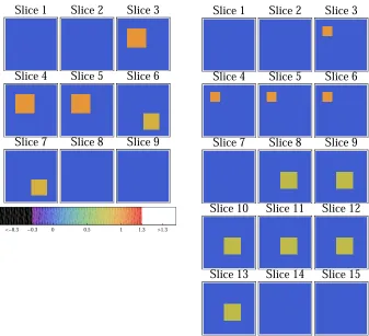
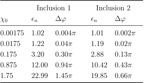
5.1 Small target susceptibilities and estimated phase shifts . . . 84

(9)

List of Figures

2.1 Illustration of the imaging geometry . . . 11

3.1 Diagram of matrix sizes . . . 29

3.2 Known elements of experimental T-matrix . . . 33

3.3 Irregular shape of known entries . . . 34

3.4 DCTMC flowchart . . . 38

3.5 Schematic illustration of fast rotations . . . 41

5.1 Targets for scalar wave diffraction simulations . . . 83

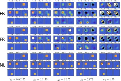
5.2 Near-field zone reconstructions for the small target . . . 94

5.3 Intermediate-field zone reconstructions for the small target . . . 96

5.4 Far-field zone reconstructions for the small target . . . 96

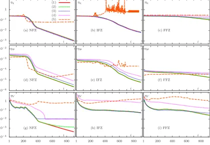
5.5 Convergence data for the small target . . . 101

5.6 Near-field zone reconstructions for the large target . . . 104

(10)

5.8 Comparison of the reconstructions of the large target with different

stopping points . . . 105

5.9 Comparison of different starting points for the iteration process . . 107

5.10 Convergence data for the case χ₀ = 0.00175 comparing the original

guess and the linear reconstruction guess . . . 109

5.11 Convergence data for the case χ0 = 0.175 comparing the original

guess and the linear reconstruction guess. . . 109

5.12 Convergence data for the caseχ0 = 1.75 comparing the original guess

and the linear reconstruction guess . . . 110

5.13 Convergence data for the case χ₀ = 0.0175 comparing the original

process and using reciprocity of sources and detectors. . . 112

5.14 Reconstructions with varying degrees ofR, the radius of row-summing114

5.15 Convergence data of η_χ for varying radii of row-summing . . . 115

5.16 Convergence data of ηχ for varying radii of row-summing, with or

without weight function . . . 116

5.17 Reconstructions with varying degrees ofR, the radius of row-summing,

with or without weight function . . . 117

5.18 Improved reconstructions for the small target in the near-field zone 119

5.19 Convergence data of η_χ comparing improved reconstructions versus

(11)

5.20 Convergence data of ηΦ comparing improved reconstructions versus

original near-field small target reconstructions . . . 121

5.21 Convergence data of comparing improved reconstructions versus orig-inal near-field small target reconstructions for χ₀ = 1.75 . . . 121

5.22 Targets for DOT simulations . . . 124

5.23 Reconstructions of the far target . . . 128

5.24 Convergence plots for the “far” target. . . 129

5.25 Reconstructions of the near target . . . 131

5.26 Convergence plots for the “near” target. . . 131

6.1 Schematic illustration of setup for toy problem . . . 133

6.2 Convergence regions of toy problem as series . . . 138

6.3 A comparison of iterative solvers with close initial guess . . . 143

6.4 A comparison of iterative solvers with far initial guess . . . 144

6.5 A comparison of iterative solvers with guess close to GN local minimum144 6.6 A comparison of iterative solvers with guess close to DCTMC local minimum . . . 145

6.7 Small target . . . 147

6.8 Noiseless reconstructions for all three methods . . . 150

6.9 Convergence data for the noiseless reconstructions from all three methods . . . 151

(12)

(13)

Chapter 1 Introduction

Inverse scattering problems (ISPs) are a topic of interest in many fields. With

ap-plications from geophysics to medical imaging, the common goal of reconstructing

one or more unknown characteristics from the produced scattered field of an object

allows one to gain knowledge of what is inside an opaque region in a

nondestruc-tive manner. This can be extremely valuable information, and modern examples

include diffuse optical tomography [3, 11], diffraction tomography [15, 21], electrical

impedance tomography [2, 13, 27], electromagnetic imaging (near-field [7, 8, 16] and

far-field [9, 53]), and seismic tomography [28, 29]. All of these methods share the

restriction that scattered field measurements can only be made on the boundary or

exterior to the object of interest.

In theory, if the scattering properties of the object are known ahead of time, it

(14)

multiple source waves scatter after making contact. This is the forward scattering

problem, which is of limited use in tomography, as the scattering effect cannot be

known ahead of time. The inverse problem is more critical, and is in general much

more difficult.

Inverse scattering problems are well known to be ill-posed [40]. As defined by

Hadamard, this implies that the inverse problem fails to have a unique solution,

fails to have a solution at all, or the solution does not depend continuously on the

measured data. It is common for an ill posed problem to suffer from more than one

of these deficiencies. When one cannot make direct measurements inside the sample

(as is the case for ISPs), it is typically impossible to uniquely determine a solution.

Moreover, once one takes into account the potentially robust noise present in any

scattering data measurements, it is clear that finding a reasonable solution is no

easy task.

To handle this ill-posedness, suitable regularization techniques must be applied.

Popular choices such as Tikhonov regularization sacrifice exactness to restore

exis-tence, uniqueness, and stability of solutions [18]. With an appropriate regularization

scheme, a reasonably precise solution can be found for many difficult ISPs.

Further complicating matters is the fact that many ISPs are nonlinear [44, 47]. A

major contributing factor to this nonlinearity is the presence of multiple scatterings.

One cannot blindly use the superposition principle to independently reconstruct

(15)

potentially strong scattering effect between the two scatterers. This nonlinearity

adds significant difficulties to any solution process, as the well-developed class of

linear solvers may not be applicable.

Linear approximations can be useful in many instances of ISPs, but many

prob-lems contain large levels of nonlinearity, and true nonlinear methods must be

em-ployed. While there are several analytic inversion approaches (such as the inverse

Born series [38, 39]) and Bayesian inference nondeterministic methods [51] that

have their merits, the class of nonlinear iterative algorithms are a popular choice

for approaching ISPs. With an iterative approach, regularization can be added as a

realization of continuous regularization strategies, or as a rule for determining the

stopping index. Three-dimensional inverse scattering problems can be a significant

computational undertaking, and iterative methods often can provide reasonable

results in a reasonable amount of computation time.

The most conventional choices of nonlinear iterative algorithms are the family

of variants on Newton’s method [25]. These methods search for a descent direction

at each iteration that moves closer to the desired result. Unfortunately, this search

for a descent direction has the serious drawback of requiring access and the use of

all available data points at each iteration. With the heavy computational workload

associated with many of these problems, one does not want to take too many data

measurements that will significantly slow down the solution process.

(16)

accurate results. As mentioned there is strong ill-posedness present due to the

re-striction on where data measurements can be made. One of the key tools to combat

this ill-posedness is the ability to make a significant number of data measurements.

In diffuse optical tomography for example, it is not totally uncommon to expect

data sets on the order of 109 to obtain acceptable resolution [12, 31, 32, 50]. Thus

with these nonlinear iterative techniques, it seems one must always balance the need

for additional data measurements to supply enough information, with the

associ-ated increase in computation time.

This thesis introduces a novel nonlinear iterative algorithm named data-compatible

T-matrix completion (DCTMC). Motivated by the need for efficient algorithms

that can solve large three-dimensional ill-posed ISPs in a reasonable amount of

time, DCTMC is not limited by the number of data measurements taken. That

is, adding additional data points does not significantly increase the computational

load of each iteration. In fact, the data set is only explicitly used once to initialize

the iterations, and the subsequent processes that utilize the data are

inconsequen-tial operation-wise in comparison with the other operations. Thus, DCTMC has

the potential to be faster and more accurate than the current choices for nonlinear

iterative methods.

The remainder of this thesis is organized as follows. We begin in Chapter 2 with

(17)

to solve the related inverse problem. Next in Chapter 3 we introduce the

data-compatible T-matrix completion algorithm, as well as many computational

short-cuts and improvements. In Chapter 4, we provide several important results

associ-ated with the linearized DCTMC algorithm. We test the DCTMC algorithm with

substantial simulations in Chapter 5 that model scalar wave diffraction and diffuse

optical tomography. Lastly, we compare DCTMC analytically and numerically to

standard nonlinear iterative methods in Chapter 6 followed by a final summary in

(18)

Chapter 2 Theory

2.1 Scattering Theory

The background information on scattering theory in this section is based on the work

in [20, 41]. The goal of any forward scattering problem is to compute the resulting

field produced by the interaction of an incident wave and an inhomogeneous object

compared to background. We state this general physical situation by

Lu(r) =q(r), (2.1.1)

where L is a linear operator, u(r) is the physical field, and q(r) is the induced

source at a location r. We are working in the frequency domain, and while both

u and q contain the frequency ω as an argument, this argument is dropped as

we consider the case of fixed frequency. The dependence between the field and

(19)

For example, varying the frequency is important in several types of time domain

problems, but for our purposes it will be ignored.

We can write L = L0 − V, where L0 is the linear operator governing the

field without an added inhomogeneous scattering region. Here, V is the scattering

potential, or interaction operator, which models the interaction between the field

and the obstacle. It is assumed that V is compactly supported in a finite scattering

volume.

Thus, absorbing the known term L0u into the induced source term q, we can

write the relationship between the field and the induced source by

Q(r) = V(r)u(r) . (2.1.2)

In this sense, the incident wavefield interacts with the potential generating the

in-duced source Q. While scattering theory can be very general, potential scattering

describes many problems of interest in electromagnetics, optics, and acoustics.

Ig-noring the vectorial nature of electromagnetic wave fields, the literature provides

the general form for the scattering potential

V(r) =k2₀[1−n2_r(r)], (2.1.3)

where n_r(r) is the relative index of refraction which measures the ratio of the index

of refraction of the scatter to the index of refraction of the background material.

That is,

n_r(r) = n(r)

n0

(20)

Keep in mind that we are still suppressing the frequency argument, which is present

iin all terms in the equation above. For a fixed frequencyω, the constant

wavenum-ber in (2.1.3)k0 is defined ask0 = (ω/c)n0(ω). In this view, the scattering potential

is completely defined by its complex index of refraction.

The field produced from the forward scattering problem must satisfy the

inho-mogeneous Helmholtz equation, that is

[∇2+k2₀]u(r) = V(r)u(r) , (2.1.5)

where we have replaced the source term on the right-hand side by (2.1.2). Reducing

the field u into a decomposition of the incident and scattered fields, we obtain

u=u_inc+u_scatt , (2.1.6)

where we conclude that the incident field satisfies the homogeneous Helmholtz

equa-tion. This is assumed despite the fact that the incident field will in all likelihood be

propagated through a background medium that is not equal to free space. In this

sense, the incident field will satisfy the inhomogeneous Helmholtz equation.

How-ever, as the source is separated from the scatter, the incident field u_inc satisfies the

homogeneous Helmholtz equation within the compact scattering region. An explicit

example of solving the inhomogeneous Helmholtz equation for the scattered field

will be provided in Section 5.1.1. For now, we will return to symbolic notation to

maintain generality.

We writeuinc =G0q, whereG0 is the unperturbed Green’s function which is the

(21)

V = 0. We will denote the complete Green’s function of the system by G=L−1.

Thus, the total field can be written as u = Gq. It is worth highlighting the fact

that G exists whenever the forward problem has a solution. Now, acting on both

sides of the equation (2.1.1) by the unperturbed Green’s functionG₀, we obtain the

Lippman-Schwinger integral equation in symbolic form

u=u0+G0V u . (2.1.7)

Rearranging terms, we can then obtain the solution for the scattered field by

uscatt= (G−G0)q =G0(I−V G0)−1V G0q . (2.1.8)

We now turn to the inverse scattering problem where we are interested in

recon-structing the scattering potential V. To have a chance of reconstructing V with a

reasonable amount of accuracy, it is imperative to have multiple views of the

scat-tering potential. That is, multiple scatscat-tering experiments must be performed with

different incident fields. Single experiments can be used for inverse source problems,

but the extra information provided from multiple scattering experiments is crucial

for the reconstruction process. To that end, we obtain data measurements by

mea-suring the scattered field at detector locations rd. Then, to obtain multiple views,

we can propagate waves through the medium from localized sourcesq(r) =δ(r−rs),

changing the location of rs for each experiment. We will denote the set of sources

by Σs and the set of detectors used by Σd. Then, by collecting the measurements

(22)

of two variables Φ(r_d,r_s). Looking back at equation (2.1.8), we see that replacing

q by each point source, the equation

G0(I−V G0)−1V G0 =Φ (2.1.9)

holds for restricted values of r and r0. That is, the operator G0 is the same

oper-ator all three times in the equation above, but each kernel G0(r,r0) has different

restrictions. For the first operator multiplication, r∈Σdandr0 ∈Ω, where Ω is the

scattering sample. The last operator multiplication is restricted by r ∈Ω,r0 ∈Σs.

Finally, the operator G0 that both has an operator multiplication and inversion is

restricted solely within the sample, r,r0 ∈Ω. Thus, the inverse scattering problem

can be stated as reconstructing the unknown interaction operator V from a data

function Φ measured outside the sample. The inverse problem is clearly nonlinear.

While Φ is theoretically measured continuously across the surfaces Σs and Σd,

it is impossible to do this in practice. One can only measure the scattered field

at a finite number of points, and likewise can only illuminate the sample from a

finite number of point sources. In this regard, the operator equation (2.1.9) must be

discretized to allow any numerical or analytical solving to take place. Thus, after

discretizing the sample, we consider the matrix equation

A(I−VΓ)−1V B =Φ . (2.1.10)

In equation (2.1.10), we have replaced the three instances of G0 by matrices of

(23)

!

d

!

s

r

d

r

s

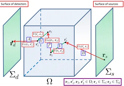
G0(rd,r01)

!"#$%&'(#')&*&%*("+ !"#$%&'(#'+(!"%&+

r

1

,

r

0₁

,

r

2

,

r

0₂

;

r

s

!

s

;

r

d

!

d

G0(r1,r2) V(r01,r1)

V(r2,r02)

G0(r02,rs)

r01

r1

r2

V

r02

V

A

B

Figure 2.1: Illustration of the imaging geometry. The matrices A, B, Γ and V

are the discretized operators in (2.1.10) and are depicted in blue frames. The

restricting and sampling of the kernels G₀(r,r0) and V(r,r0) are demonstrated by

the endpoints of the arrows. The multiple scattering depicted corresponds to the

second order term G0V G0V G0in the formal power-series expansion of the left-hand

side in (2.1.9). Note that in the local limit of the potential V(r,r0) the two green

arrows contract to two vertexes at r1 =r01 and r2 =r02.

manner. A is restricted from the detectors to the sample, B is restricted from the

sources to the sample, and Γ is restricted within the sample itself. An example of

this is shown in Figure 2.1. While the slab geometry example in this figure is the

main geometric setup we will be investigating in our later simulations, the above

formulation is general and does not require any specific shape for the surface of

detectors or sources, or the sample. The only physical requirement is that there is

(24)

Equation (2.1.10) is not only general with respect to the geometric setup of

the problem and the discretization choices, but is very general in regards to its

application to scattering theory. The geometry matrices A, B, and Γ are all

theo-retically known, and encompass all of the information of the physical model. Since

the elements of the matrix Φ are all acquired experimentally, the only unknown in

(2.1.10) is the scattering potential V. It is important to note that this equation

cannot be solved simply by matrix inversion, as the matrices A andB are typically

of low rank. In fact, the invertibility of these matrices coincides with performing

measurements within the sample, which is a strict violation of the problem. We

now turn to methods for recovering the interaction operator V.

2.2 Nonlinear Reconstructions

Oftentimes, a linearization of the ISP is an acceptable method for solving this inverse

scattering problem. For these methods, a linearizing transformation is applied to

the data function on the right-hand side of (2.1.10) to simplify the forward problem

to be linear in terms of the unknown interaction matrix V, namely

AV B=L[Φ] . (2.2.1)

Moreover, it is conventional to assume that the interaction matrix is strictly

diag-onal, and such by combining the geometry matrices A and B into the matrix K

(25)

vector ψ, one obtains the linear equation

Kv =ψ . (2.2.2)

This equation can then be solved for v using any linear equation solver. We will

discuss more linearizing techniques in Sections 4.1 and 5.1.

Another approach to solving inverse scattering problems is to use one of

sev-eral known nonlinear techniques for reconstructing the interaction matrix. These

approaches intend to reconstruct the images with greater accuracy as compared to

linear solvers which make approximations that can significantly reduce the accuracy

of the model. However, nonlinear methods are more computationally intensive than

linear solvers. For that reason, there are many practical scenarios when a linear

re-constructions are acceptable. But when the results obtained from the linearization

of the ISP is not worthy of its application, one must increase the computational

load and use a nonlinear method.

The most popular approach to solving nonlinear inverse scattering problems is

to use Newton’s method or one of its variants. This section will review the idea

behind these mainstream approaches. These methods are reviewed in more detail in

[1, 17, 30]. However, it is worth keeping in mind alternative nonlinear methods such

as the inverse Born series, where the reconstruction is an analytically computable

result directly from the data, and several non-deterministic approaches based on

Bayesian inference.

(26)

of equation (2.1.10) and rewrite the ISP in the form F[v] = 0, where v are the

diagonal entries of V and F is the nonlinear functional that relates the scattering

potential to the data. This can be alternatively written as AT B = ˜F[v] which

can more clearly elucidate the relationship the nonlinear functional ˜F has with the

data. From here, one thinks of the inverse scattering problem as an optimization

problem. The solution ˆv is found by minimizing an objective function

ˆ

v = arg min

v Ψ(v). (2.2.3)

In most cases, it is common to treat this objective function Ψ as the statement of

a nonlinear least squares problem, that is

Ψ(v) =

Ns

X

i=1

Nd

X

j=1

[Φc(v)−Φm] , (2.2.4)

where Φm is the measured data for specific source and detector pair, and Φc(v)

is the calculated data for that same pair given a scattering potential within the

vector v. We denote the number of sources and detectors used as Ns and Nd

respectively. Then starting from an initial guessv₀, the forward problem for Φc(v₀)

is calculated, and then based on the specific minimization scheme, our guess is

updated by vk+1 =vk+γkdk, where dk is a descent direction, and γk is a step size.

Oftentimes in the literature γ_k = 1, as the step size is typically independent of the

method used to determine the descent direction. However, one can always add an

optimization step that conducts a line search for a useful value of γk. That is,

γk= min

(27)

We will now mention some of the most commonly used methods to determine the

direction dk.

2.2.1 Landweber Iteration

Landweber iteration is a special case of steepest descent, in which constraints are

placed on the step size γk. Thus, dk =−∇Ψ(v). Numerically, defining the residual

column vector R(v) with entries

ri(v) = Φci(v)−Φmi , (2.2.6)

allows us to express the gradient of the objective function as the product

∇Ψ(v) =J(v)TR(v), (2.2.7)

where J is the Jacobian matrix defined as

J(v) =          

∂r1(v)

∂v1 . . .

∂r1(v)

∂vN

..

. . .. . . .

∂rM(v)

∂v1 . . .

∂rM(v)

∂vN           . (2.2.8)

Here, N is the number of discretized elements in the sample, and M = NdNs

is the total number of data points. Thus, Landweber iteration can be succinctly

summarized as

vk+1 =vk−J(v)TR(v) . (2.2.9)

While steepest descent algorithms are well known for converging from very far

(28)

is rarely used directly in practice.

2.2.2 Gauss-Newton Method

A faster and more popular method for nonlinear optimization is the Gauss-Newton

iteration method. While steepest descent used only first-order derivatives,

Gauss-Newton uses an approximation to the second derivative. We begin with the

first-order Taylor approximation to the gradient of the objective function

∇Ψ(v_k₊₁) = ∇Ψ(v_k+d_k)≈ ∇Ψ(v_k) +∇2_Ψ(_v

k)dk . (2.2.10)

Thus as the objective function is minimized when this equation is equal to zero, we

are interested in solving the set of equations

∇2Ψ(v_k)d_k=−∇Ψ(v_k) , (2.2.11)

for the Gauss-Newton direction dk. The term∇2Ψ(vk) is the Hessian operator and

can be calculated as

∇2Ψ(vk) = 2J(vk)TJ(vk) +

M

X

m=1

Nv

X

i=1

Nv

X

j=1 ri(v)

∂rm(v) ∂vi∂vj

. (2.2.12)

In practice, the second term requires a very lengthy calculation, and is in fact

typically much smaller than the first. Therefore, Gauss-Newton method uses the

approximation

∇2_Ψ(_v

(29)

This combined with the previous result∇Ψ(v_k) = 2J(v_k)TR(v_k), we obtain a set of

linear equations to solve for the search direction, namely

J(vk)TJ(vk)dk =J(vk)TR(vk). (2.2.14)

Gauss-Newton can converge much quicker than steepest descent, but fails to

con-verge for initial guesses not close to the desired result. However if an initial guess

is sufficiently close, convergence is quadratic.

2.2.3 Levenburg-Marquardt Method

The Levenburg-Marquardt method is a popular nonlinear iterative algorithm that

balances the benefits of both steepest descent iteration and Gauss-Newton method.

In its purest form, a positive diagonal matrix is added to the approximation to the

Hessian on the left-hand side of (2.2.14). Most commonly this diagonal matrix is

chosen to be a multiple of the identity matrix, giving the set of linear equations

governing this method to be

(J(vk)TJ(vk) +λkI)dk =J(vk)TR(vk) . (2.2.15)

This choice closely resembles the well-known Tikhonov regularization and is in fact

equivalent to iteratively regularized Gauss-Newton. For very small values of the

damping parameterλk, the direction is clearly very close to the direction obtained by

pure Gauss-Newton. However, larger values of λk suppresses the second derivatives

(30)

is closer to steepest descent. Thus, the choice of λ_k can be modified each iteration –

if it is known that our intermediate result is reasonably close to correct, λk should

be made small to have near quadratic convergence behavior a la Gauss-Newton. If

we can be reasonably sure we are far away, a larger value of λ_k would be preferred

for a larger convergence radius.

2.2.4 Nonlinear Conjugate Gradient

The last common nonlinear reconstruction technique we will review is nonlinear

conjugate gradient. Regular conjugate gradient is a linear iterative method for

solving symmetric positive definite linear systems. Convergence is guaranteed for

the linear case in at most n iterations, where n is the size of the system, and

acceptable results can be found much faster depending on the spectrum of the

matrix involved. For completeness sake (and as this algorithm is used later in the

simulated linear reconstructions) this algorithm for solving the equation Kv = ψ

goes as follows for an initial guess v0:

1. r0 =Kv0−ψ

∆v0 =−r0

2. While krkk> do

(a) αk = r

T krk

∆vT kK∆vk

(31)

(c) r_k₊₁ =r_k+α_kK∆v_k

(d) βk+1 =

rT k+1rk+1

rT krk

(e) ∆vk+1 =−rk+1+βk+1∆vk; k =k +1

Nonlinear conjugate gradient method can then be directly obtained from its linear

counterpart by removing all instances of the residual rk from the above algorithm

and replacing it with ∇Ψ(vk).

2.3 T-matrix

The T-matrix is defined as the operator that relates the complete and unperturbed

Green’s functions through the Dyson equation

G=G₀+G₀T G₀ . (2.3.1)

A simple inspection of equation (2.1.8) solves for this operator as

T = (I−V G0)−1V . (2.3.2)

Another interesting way of looking at the T-matrix is to define the transition

op-erator which maps incident waves into the product of the interaction opop-erator and

the total wavefield [14, 46]. That is,

(32)

and if we multiply both sides of the Lippman Schwinger (2.1.7) equation by the

scattering potential V, we obtain

T u0 =V u0+V G0T u0 , (2.3.4)

or equivalently

T =V +V G0T (2.3.5)

Again solving this equation for T we arrive precisely at the definition in (2.3.2).

From the definition of the transition operator, one can conclude that the scattering

amplitude outside of the sample is proportional to the boundary value of the

T-matrix over a sphere. Thus, scattering amplitude can be determined directly from

the T-matrix, but not vice versa. Clearly the T-matrix completely determines the

scattering operator through the one-to-one correspondence in (2.3.2), but merely

knowing the scattering amplitudes only determines the scattered field outside of the

sample. Thus, one can think of the inverse scattering problem as computing the

T-matrix from some analytic continuation of the scattering amplitudes. However,

there is no stable method to accomplish this.

As an actual discretized matrix, the relationship between the T-matrix and V

is written as

T = (I−VΓ)−1V =V(I−ΓV)−1 . (2.3.6)

Clearly, the T-matrix is symmetric. The inverse operation in equation (2.3.6) is

(33)

From (2.3.6), we can calculate that

V = (I+TΓ)−1T =T(I+ΓT)−1 . (2.3.7)

Thus, we have a one-to-one correspondence between the transition matrix and the

interaction matrix. Knowledge of either of these matrices fully determines the

(34)

Chapter 3 The Data-Compatible T-matrix

Completion Algorithm

3.1 Motivation

We now turn towards the crux of this these – introducing the novel nonlinear

itera-tive method, data compatible T-matrix completion. Before detailing the specifics of

the algorithm, it is worth discussing the desire for additional methods to approach

nonlinear inverse scattering problems. All of the methods reviewed in Section 2.2

calculate an objective function which depends on all available data measurements,

and is subsequently minimized using one of the previous schemes. In its naive form,

computationally implementing any of these methods at least require storage of the

(35)

andN_v is the number of discretized elements one wants to reconstruct. And then for

say Gauss-Newton, one also requires the matrix multiplication JTJ, which requires

O(M2Nv) operations. This calculation quickly becomes unwieldy as the number of

data measurements increases. This is clearly unwanted, as one of the major tools

we have to solve inverse scattering problems is the ability to conduct multiple

ex-periments and obtain very large data sets. However, with traditional methods one

must balance the benefits from additional data measurements versus the increased

computational workload.

It would be dishonest to leave out the fact that there exist more efficient methods

for generating and multiplying these large Jacobian matrices, and thus run faster

than O(M2Nv). Adjoint methods such as in [4, 5, 43] can take advantage of the

sparse nature of the Jacobian matrix in a manner where the Jacobian matrix is never

explicitly computed. But while there are certainly computational improvements one

can make when using these Newton methods, one cannot escape the fact that the

computational workload increases as our data set increases as well.

There is substantial evidence that inverse scattering problems of interest require

strongly overdetermined data sets in order to obtain accurate results [36, 37]. For

example, to obtain optimal lateral resolution for diffuse optical tomography in the

slab geometry with 100×100 grid cross-sections, one needs on the order of 300×300

panels of sources and detectors on either side of the sample. This set up produces

(36)

size of the discretization mesh, and is the limiting factor for mainstream nonlinear

approaches. This relative magnitude of the size of the overdetermined data set

holds for many other ISPs of interest.

There has been a great deal of interest in both acquiring these large data sets,

and experimentally determining the optimal size of data sets for DOT [6, 31, 50].

Noise and severe ill-posedness can warrant a reduction in the optimal size of the data

set, as one can reach the limit of resolution, and especially noisy data measurements

are better off left discarded. However, the majority of these works use linearized

reconstruction techniques to be able to handle the large data sets efficiently. Thus,

it is certainly desirable to develop nonlinear techniques that will forgo these linear

approximations that reduce accuracy, but can still reconstruct from large data sets

with reasonable computing time.

This is the main goal of DCTMC – to present a nonlinear solver in which

in-creasing the size of the data set has a negligible impact on computation time. The

descriptions of the Newton type solvers in Section 2.2 are very clear in that the

unknown interaction matrix from the forward matrix equation (2.1.10) is treated

as being strictly diagonal and can thus be reduced to a column vector. This comes

from the theory of locality, which states that certain physical properties or events

at a specified point r are only influenced by the field present within a finite radius

(37)

never zero, the radius of influence ` is typically small enough (often on the atomic

scale which is much smaller than any discretization mesh), that the forced diagonal

structure of V is accurate.

DCTMC relaxes this locality restriction, and allows our iterative process to

search for nonlocal interaction operators as well. For example, Ohm’s law in local

electrodynamics isJ(r) =σ(r)E(r). Relaxing this to nonlocal electrodynamics, the

current density J(r) is given by

J(r) = Z

V(r,r0)E(r0)d3r0 , (3.1.1)

where V is the integral interaction operator as in (2.1.2). Now we consider the

Calderon problem where we want to find the conductivity σ(r) from voltage drop

measurements taken after two electrodes inject direct current. Finding a nonlocal

kernel V(r,r0) from 3.1.1 that is consistent with the voltage drop measurements

can be simple as this problem is very underdetermined – the degrees of freedom of

V(r,r0) is much larger than the size of the data set. But for the exact same reason,

V(r,r0) cannot be determined uniquely. What we have accomplished so far by

generalizing the linear relationship between the current density and electric field to

a nonlocal setting is the ability to find many solutions that are compatible with the

data. The question remains, how can we narrow down to our desired solution? Keep

in mind that our generalization to the nonlocality of V was only a mathematical

trick, we still expectV to be local to some degree, that isV(r,r0)→0 when|r−r0|>

(38)

conductivity can be obtained from the integral operator by σ(r) = R

V(r,r0)d3r0.

Our search out of our data consistent solutions is narrowed down to a search for an

approximately diagonal nonlocal kernel V(r,r0). The concept for DCTMC can be

summarized as:

(1) An initialization step where a class of kernels V(r,r0) that are compatible

with the data is formed. This initialization is the only place when the data

measurements are explicitly used. Moreover, the size of the data set is not a

limiting factor for defining this class of data compatible solutions.

(2) Then we iteratively reduce the off-diagonal norm of V(r,r0) while ensuring

that all iterations of V(r,r0) remain compatible with the data.

(3) Once the ratio of the off-diagonal and diagonal norms ofV(r,r0) is sufficiently

small, we have found our diagonally dominated data-compatible interaction

operate. We then compute the local interaction σ(r) =R V(r,r0)d3r0. This is

the final solution to the nonlinear ISP.

While this motivation was stated for electrical impedance tomography, its statement

is very general and can be applied to many other inverse scattering problems. The

fact that (1) above is the only time the data is used (and is not limiting) highlights

the potential advantages of this algorithm.

Lastly of note, the T-matrix from Section 2.3 plays a crucial role in the DCTMC

(39)

problems [33, 52]. These methods are source and detector independent, as the

computation of the T-matrix gives the forward solution for any source and

de-tector arrangement. The mainstream Newton approaches typically utilize finite

difference and finite element methods for the forward problem, which must be run

for each source independently. However, finite element methods generate sparse

matrices which allow for some of the reductions mentioned required for Jacobian

calculations. The trade off for working with source/detector independence is that

computing the T-matrix as in (2.3.6) requires inverting a dense matrix. This

one-to-one correspondence between the interaction operator V and the T-matrix plays

an important role in DCTMC.

3.2 The Experimental T-matrix

We return to the discretized forward equation for the scattering problem

A(I−VΓ)−1V B =Φ , (3.2.1)

but now substituting in equation (2.3.6) to obtain the forward equation

AT B =Φ , (3.2.2)

which is a linear equation in T. It is worth taking some time to discuss the relative

sizes of all matrices in equation (3.2.2). The volume is discretized into Nv voxels,

(40)

it is clear that the inequality

N_s, N_d N_v N_sN_d (3.2.3)

must hold if there is any hope of solving the inverse problem with reasonable

accu-racy. The first inequality is generally true due to the nature of most problems of

in-terest, namely that it is impossible to take enough useful measurements to perfectly

determine a solution. The second inequality states that we need an overdetermined

system to handle the ill-posedness involved. So while this inequality holds true in

general, it is useful to consider the order of the values used throughout this paper.

As in the setup in Fig. 6.1, let the measurement planes Σ_s and Σ_dbe identical, with

both sources and detectors scanned on L×Lsquare grids. The sample is discretized

with the same pitch as the source/detector grids on an L×L×L cubic grid. Then,

N_s =N_d=L2,N_v =L3, andN_sN_d=L4, which certainly satisfies condition (3.2.3)

for reasonable values of L.

The dimensions of all matrices in equation (3.2.2) are shown in Fig. 3.1. For

all of the reasons mentioned, we can assume that A and B are not invertible.

However, since we have rewritten the forward equation to be linear equation in

our fundamental unknown T, we can fully utilize the knowledge of pseudoinverses.

This will lead us to the definition of the experimental T-matrix, which is the central

concept to DCTMC.

The idea is to find a condition on T that completely satisifies equation (3.2.2).

(41)

T

=

â

N_v N_v Nv Nv

N

_d

N

s

N

_s

N

_d

B

A

Figure 3.1: Schematic block diagram of equation (3.2.2). Nv is the number of

discretized voxels, while Nd and Ns are the numbers of detectors and sources

re-spectively.

A and B. That is,

A=

Nd

X

µ=1

σ_µAf_µA g_µA

, B=

Ns

X

µ=1

σ_µBf_µB g_µB

, (3.2.4)

where σA_µ are the singular values of A, and f_µA

are the left singular vectors of A

of length Nd and

g_µA

are its right singular vectors of lengthNv. This is similar for

B, but with the left singular vectorsf_µB

being of length Nv and the right singular

vectors g_µB

being of length Ns. Note that the summations in (3.2.4) have upper

indicies of Nd and Ns, due to our assumption that Nd, Ns ≤Nv (all singular values

of larger index thanNdorNsare identically equal to zero). Now using orthogonality

of singular vectors and rearranging our forward equation, we obtain the entrywise

condition

(42)

where we have the following entrywise definitions:

˜

Tµν ≡

g_µA|T|f_νB

, 1≤µ, ν ≤Nv ; (3.2.6a)

˜

Φµν ≡

f_µA|Φ|g_νB

, 1≤µ≤Nd , 1≤ν ≤Ns . (3.2.6b)

We now letRAbe theNv×Nvunitary matrix formed by the column singular vectors

|gA

µiand RB be theNv×Nv unitary matrix formed by the column singular vectors

|fB

µi. Then, the first line of equation (3.2.6) implies with the unitary property that

˜

T =R∗_AT RB and T =RAT R˜ ∗B . (3.2.7)

Note that even though this transformation from T to ˜T is invertible, it is not a

conventional rotation due to the fact that RA 6= RB in general. We now call the

matrixT that has been used thus far the T-matrix inreal-space representation, while

the “rotated” matrix ˜T is named the T-matrix insingular-vector representation. We

could name Φ˜ and Φsimilarly, albeit using different unitary matrices (of dimension

Nd×Nd and Ns×Ns). But to avoid confusion, since Φ˜ is not a recurring aspect of

the DCTMC algorithm, we refrain from explicitly defining these “rotations”.

Returning to the equivalent singular-vector representation forward equation

(3.2.5), we see that we can numerically reduce this constraint to

˜

Tµν =

           1 σA µσνB

˜

Φµν , if σµAσνB > 2 ;

unknown , otherwise .

(3.2.8)

where we have used the conventional notation that σ_µA and σ_µB are equal to zero

(43)

reg-ularization parameter to deal with numerical imprecisions. With infinite precision,

equation (3.2.8) results in NsNd known values, but for an appropriate choice of

larger than the smallest positive floating-point constant of computational precision,

it is certainly possible for this equation to give less than N_sN_dknown values in the

T-matrix in singular-vector representation.

However many known entries results from equation (3.2.8) summarizes the

en-tirety of our knowledge based solely on the data. But we know these entries are

correct in singular-vector space with great certainty. In fact, since these entries fully

(or nearly, depending on the choice of) represent the data, any choice or

modifica-tion to the unknown values will have negligible impact on the error of the forward

equation (3.2.2) when the T-matrix is rotated back to real-space. This is precisely

our definition of data-compatability: a T-matrix is called data-compatabile if when

it is rotated to the basis of singular functions, it agrees with all known values from

equation (3.2.8).

In general, we can expect this equation to result in a number of known entries

not much less than or equal to N_sN_d. However, from inequality (3.2.3), we know

that NsNd Nv2, which implies that we only know a very small number of the

total entries of ˜T. For our previous estimated values of these dimensions, we have

N_sN_d/N_v2 = 1/L2, which is certainly a small fraction of known entries for large L.

We can arrange the singular values of A and B in descending order, and such the

(44)

M_A×M_B, where M_A ≤ N_s and M_B ≤ N_d. This is schematically shown in Figs.

3.2. The region of known elements can be of a general shape contained in this

rect-angular block, but we will assume it is rectrect-angular. Furthermore, in all numerical

simulations, the region was indeed rectangular. It is not complicated to include

irregular shapes (see Figure 3.3), but it adds nothing to the discussion.

We can now define the experimental T-matrix Texp as the matrix that satisfies

the forward equation (3.2.2) in the minimum norm sense with smallest norm kTk₂.

We can calculate Texp in one of two ways. The first method, which was hinted at

before, is to calculate

T_exp =A+ΦB+ , (3.2.9)

where A+ and B+ are the Moore-Penrose pseudoinverses. Then to obtain ˜T_exp in

singular-vector space, one needs to perform the necessary rotation as in equation

(3.2.7). An equivalent method is to work directly in singular-vector representation,

defining ˜ Texp µν =            1 σA µσνB

˜

Φµν , if σµAσνB > 2 ;

0 , otherwise .

(3.2.10)

which is setting all unknown entries to be identically equal to zero. It is worth

noting that even though ˜Texp is sparse, the same is not necessarily true of Texp.

Perhaps even more important to note, is the fact that by this definition T_exp is

not necessarily symmetric, even though it is theoretically known that the correct

(45)

T

à

exp

=

ûA_öûB_÷

à

ö ÷

T

à =

!"#"$%"

!"#"$%" ûA_öûB_÷

à

ö ÷

MA

MB

M_A

M_B

Figure 3.2: Left panel: Known elements of ˜T in singular-vector representation

computed from the data by using (3.2.8) are organized inside the shaded block in the upper left-hand corner. Elements outside of this shaded block are not known

and completely independent of the data. Right panel: The experimental T-matrix,

Texp, the minimum norm solution to (3.2.2). This is equivalent to setting the

un-known elements of ˜T to zero.

inherent to the algorithm, we can easily ensure symmetry. We are now ready to

proceed to defining the basics of the iterations.

3.3 Iteration Cycle

There are two main conditions to be met:

(i) The T-matrix must be data-compatible

(ii) The corresponding V-matrix must be diagonally dominated

Our goal is to “complete” the matrix ˜T in singular-vector space by filling in the

unknown elements in a way that the corresponding interaction matrix V in real

space is diagonally dominant. By using the one-to-one correspondence between the

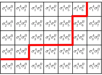
T-matrix and the interaction matrix V, and the invertible rotations between real

(46)

ûA 1û B 1 û A 1û B 2 û A 1û B 3 û A 1û B 4 û A 1û B 5 û A 1û B 6 û A 1û B 7 ûA 2û B 1 û A 2û B 2 û A 2û B 3 û A 2û B 4 û A 2û B 5 û A 2û B 6 û A 2û B 7 ûA 3û B 1 û A 3û B 2 û A 3û B 3 û A 3û B 4 û A 3û B 5 û A 3û B 6 û A 3û B 7 ûA 4û B 1 û A 4û B 2 û A 4û B 3 û A 4û B 4 û A 4û B 5 û A 4û B 6 û A 4û B 7 ûA 5û B 1 û A 5û B 2 û A 5û B 3 û A 5û B 4 û A 5û B 5 û A 5û B 6 û A 5û B 7

Figure 3.3: A more general shape of known elements of the experimental T-matrix, as compared with Figure 3.2. The elements above the thick red line satisfy the

condition σ_µAσ_νB > 2. Assuming that the singular values σA_µ and σ_µB are arranged

in the descending order, the boundary line can only go from left to right and from bottom to top if followed from the left-most boundary of the matrix. One can easily

obtain a rectangular shape by excluding the elements σ₄Aσ₁B,σ₄Aσ₂B, andσ₁Aσ₆B, but

this is not necessary.

by alternatively ensuring conditions (i) and (ii).

We now explicitly define a number of operators that will ease in the description

of the algorithm. We letT[·] be the nonlinear operators that computes the T-matrix

from a given interaction matrix by the previous definition (2.3.6)

T[V] = (I−VΓ)−1V , (3.3.1)

which is also invertible (as discussed in Section 2.3) with the form

T−1[T] = (I +TΓ)−1T . (3.3.2)

Note that both of these functionals have Γ as a parameter, and can act on any

Nv ×Nv matrix. However, they are only intended to be used for the appropriate

(47)

and singular-vector representations and its inverse R−1_[_·_{] by}

R[T] =R∗_AT R_B , R−1[ ˜T] =R_AT R˜ _B∗ . (3.3.3)

Again, these operators can act on any N_v×N_v matrix, but have been written with

the parameter of intended use. The definition of this operator also presupposes that

the rotation matrices have already been calculated, and thus the SVD representation

of A and B. With these same assumptions, we define the masking operators M[·]

and N[·]:

M[ ˜T]

µν ≡         

0, σ_µAσ_νB> 2 ;

˜

Tµν , otherwise .

N[ ˜T]

µν ≡          ˜

Tµν , σµAσνB > 2 ;

0, otherwise .

(3.3.4)

with the point that M[ ˜T] +N[ ˜T] = ˜T. Then the method of enforcing

data-compatibility of ˜T can be defined through the overwriting operator O[·] by

O[ ˜T]≡ M[ ˜T] + ˜Texp = ˜T − N[ ˜T] + ˜Texp . (3.3.5)

The operator literally leaves all “unknown” elements unchanged, and forcibly

over-writes the “known” entries.

Finally, we define the operatorD[·], which calculates the diagonal approximation

to an Nv ×Nv matrix. We will begin by defining this operator by

D= (D[V])_ij ≡δijVii , (3.3.6)

which is perhaps the simplest method of defining a related diagonal matrix by

(48)

in a similar manner. We can certainly choose alternate definitions forD[·] andO[·],

which we will later discuss and justify our final choices. For now, overwriting and

diagonalizing are done by forcibly changing any entry that is not desired.

With these definitions in hand, we can now elaborate on the iterative algorithm

DCTMC. We assume that the SVD decompositions of the geometry matricesAand

B have been precomputed, along with the experimental T-matrix ˜Texp. Let k = 1,

and our initial guess ˜T₁ = ˜T_exp. Then the algorithm runs as follows:

1: Tk=R−1[ ˜Tk]

This transforms the T-matrix from singular-vector to real-space

representa-tion. Both ˜Tk and Tk are data-compatible.

2: Vk=T−1[Tk]

This gives k-th approximation to the interaction matrix V. V_k is

data-compatible but not diagonal. Compute the off-diagonal and diagonal norms

of Vk. If the ratio of the two is smaller than a predetermined threshold, exit;

otherwise, continue to the next step.

3: Dk =D[Vk]

Compute the diagonal approximation to Vk, denoted here by Dk. Dk is

diag-onal but not data-compatible.

4: T_k0 =T[Dk]

(49)

T_k, T_k0 is no longer data-compatible.

5: ˜T_k0 =R[T_k0]

Transform T_k0 to singular-vector representation. Here ˜T_k0 is still not

data-compatible.

6: ˜Tk+1=O[ ˜Tk0]

Advance the iteration index by one and overwrite the elements of ˜T_k0 that are

known from data with the corresponding elements of ˜Texp. This will restore

data-compatibility of ˜Tk+1. Then go to Step 1.

These steps illustrate a method for iteratively ensuring data-compatibility of the

T-matrix and diagonal dominance of the interaction matrix V. A flowchart of these

iterations is shown in Figure 3.4. While these enforcements are “exclusive or” in

the boolean sense that only one of them is guaranteed to be true at any point in

the algorithm, the goal is that convergence will lead to an acceptable result on both

fronts.

3.4 Computational Complexity and Shortcuts

In terms of computational complexity, Steps 1, 2, 4, and 5 are dominant, all with

complexityO(N_v3). In this section however, we will present computational shortcuts

to reduce the number of steps with complexity O(N_v3). The first shortcut for fast

(50)

!"!#$%&'!"()*+,-#&!".(/ 0+'.+1+2"!"(%23,45 k

T

!"!#$%&'!"()*+,-#&!".(/ 0+'.+1+2"!"(%23,04 k

T

(!6%2!*,(2"+.!$"(%2#$%&'!"(# )*+,-#&!".(/

0+'.+1+2"!"(%23,04

T

k

(!6%2!*,(2"+.!$"(%2#$%&'!"(# )*+,-#&!".(/

0+'.+1+2"!"(%23,45

T

k

!"!#$%&'!"()*+ (2"+.!$"(%2,&!".(/ 7%88#9(!6%2!*: 0+'.+1+2"!"(%23,04 k

V

(!6%2!*,(2"+.!$"(%2, &!".(/ 72%",9!"!#$%&'!"()*+: 0+'.+1+2"!"(%23,04 k

D

!"#$%&$'()'*+,$'-"$+$."/,

!"#$%&$'0)'*+,$'T D

+/'

T

!

1+$+ *.#,$'.$2#+$."/ &3,24&2/$ .$2#+$."/, 51'"6'A+/7'B

1.Rà1

2.T à1

3 .

D

4.T

8 ! 2 '9 " $$ :2 / 2 %;

5 .

R

6 .

O

k

+ 1

<=.$'.6'%"/7.$."/ .,'>2$

Figure 3.4: Basic flowchart of the DCTMC iteration process for the case when

the iterations start with an initial guess of ˜T_exp. The operations for the numbered

(51)

implementation. The second shortcut which reduces computation time from the

T-matrix to the interaction matrixV is certainly useful for the definition presently

used of D[·] in (3.3.6), but may be needed to be eschewed when using alternative

definitions for the diagonal matrix approximation operator.

3.4.1 Fast Rotations and Data-Compatibility

The first shortcut combines steps 5, 6, and 1 into one step that enforces

data-compatibility by overwriting without rotating all entries to singular-vector space

and back. These steps are listed below, with their computational complexity as

well as their complexity based on the estimated values with discretization into grid

size L.

5 : T˜_k0 =R[T_k0] O(N_v3) =O(L9) ,

6 : T˜k+1 =O[ ˜Tk0] ≤O(NdNs) =O(L4) ,

1 : T_k₊₁ =R−1_{[ ˜}_T

k+1] O(Nv3) =O(L9) .

Steps 1 and 5 are obviously the dominant steps, with Step 6 only needing to access

and overwrite a maximum ofNsNdentries (and potentially less depending on desired

precision). It is natural to combine these three steps, due to the fact that the

bookend rotations are linear. Combining these three steps in one results in

Tk+1 =R−1[O[R[Tk0]]] =R

−1h_R_[_T0

k]− N[R[T

0

k]] + ˜Texp

i

(52)

where the second equality has inputted the second definition of O[·] in (3.3.5) and

the fact that R[Texp] = ˜Texp. Now we can distribute the operator R−1 across due

to linearity, which results in the expression

Tk+1 =Tk0 +Texp − R−1[N [R[Tk0]]] . (3.4.2)

This expression is identical to Steps 5, 6, and 1, but we still need to be able to reduce

R−1_[_N _[_R_[_T0

k]]] to show any computational improvements. This is not difficult, as

(3.4.2) has replaced O[·] in (3.4.1) with N[·], which turns any matrix into a sparse

matrix. Therefore, it is reasonable to expect that R−1_[_N_[_R_[_T0

k]]] can be computed

in fewer than O(N_v3) operations.

Let us first consider the operation N[R[T]]. As the masking operator N sets

all entries not in the upper left MA×MB submatrix to zero, there is no need to

calculate all entries in the rotation R[T]. Therefore we define the Nv ×MA

ma-trix PA by the first MA columns of RA, and similarly PB by the first MB columns

of RB. Then, N[R[T]] = PA∗T PB which now has computational complexity of

O(min(MA, MB)Nv2) which is a reduction over the original computational

complex-ity of O(N_v3) by a minimum ofO(L) under our estimates. Identical reasoning allows

us to expand to the full expression

R−1[N[R[T_k0]]] =PA(PA∗T PB)PB∗ , (3.4.3)

which has the same computational complexity of O(min(MA, MB)Nv2). It is clear

(53)

= â â

T

P

ã

A

P

B

= â â

T

R

ã

A

R

B

R

_[

T

_]

N

_[

R

_[

T

_]]

N

M_A

M_B

0 0

0 ₀

0

MA

MB

Figure 3.5: Schematics of computing N[R[T]]. Matrices PA and PB are obtained

from RA and RB by setting all columns to zero except for the first MA and MB

columns, respectively.

any sense. Therefore, it would be inefficient to premultiply these matrices and set

QA = PAPA∗ and QB = PBPB∗ and calculate QAT QB. Using this premultiplication

would clearly still have complexity O(N_v3). Therefore, the evaluation of (3.4.3)

should be calculated in the order implied by the parentheses to gain an improvement.

Putting all of this together, we obtain the shortcut for fast rotations combing Steps

5, 6, and 1 by

Tk+1 =Tk0 +Texp−PA(PA∗T

0

kPB)PB∗ . (3.4.4)

With this shortcut, it is no longer necessary to store the full matrices of RA and

RB in memory. We only need to precompute and store PA and PB. Since Texp is

(54)

3.4.2 Fast

T

→

D

Transformation (Option 1)

We now consider another shortcut that will quickly calculate the related interaction

matrix V to the T-matrix and simultaneously find its diagonal approximation D.

This shortcut can be thought of as not a pure shortcut to the algorithm, but as an

alternative definition to the closest diagonal approximation operator D[·] that runs

faster. Our previous definition was to compute V that perfectly corresponds to T,

but is most likely not diagonally dominated. Then we set all off diagonal terms to

zero to arrive at our diagonal approximation. Put alternatively, we seek a diagonal

matrix D that minimizes kV −Dk2. However, we can also search directly for the

nearest diagonal matrix D that corresponds to T. From (2.3.7), we have

T =D+DΓT , (3.4.5)

which we can solve as a classical minimization problems, stated as

min

D diagonalkT −D−DΓTk2 . (3.4.6)

We can explicitly solve problem (3.4.6) to arrive at the solution:

Dij =δij

Tii+ [(ΓT)

∗

T]_ii

1 + [(ΓT)∗+ (ΓT) + (ΓT)∗(ΓT)]_ii . (3.4.7)

While we have arrived at a nice closed-form solution to (3.4.6), at first glance it

seems like this evaluation still requires O(N_v3) operations, which is not an

improve-ment over the original method which required the inverse an Nv×Nv matrix. The

issue seems to be the calculation of the product ΓT, however, we are able to

(55)

the matrix Λ = ΓT, and look back at the computational shortcut for fast rotations

as stated in (3.4.4). We can multiply both sides of the equation by Γ to obtain

ΓTk+1 =ΓTk0 +ΓTexp−ΓPA(PA∗T

0

kPB)PB∗ , (3.4.8)

or using the natural extension of the definition of Λ,

Λk+1 = Λ0k+ Λexp−(ΓPA) (PA∗Tk0PB)PB∗ . (3.4.9)

The matrix ΓPA can be precomputed at the start, as well as the matrix Λexp =

ΓTexp, so the only remaining issues is how to obtain Λ0k. If this matrix can be easily

obtained, then the computational complexity of (3.4.9) is identical to the complexity

of the previous shortcut, namely O(min(MA, Mb)Nv2). It is a reasonable question if

the computation of Λ0_k requires a new matrix multiplication, due to the fact that

ΓT_k0 has not been used previously. However, it can be precomputed without any

additional cost in the previous step of the algorithm. From the definition of T[·] in

(3.3.3), we have

T_k0 =D_k(I−ΓD_k)−1 . (3.4.10)

which results in

Λ0_k =ΓDk(I−ΓDk)−1 = (I−ΓDk)−1−I , (3.4.11)

when both sides of (3.4.10) are left-multiplied by Γ. Thus,as we already need to

calculate this inverse matrix, we are able to obtain Λ0_k simply by subtracting off of

(56)

1: Compute the product∆_k≡ΓD_k, which is fast because D_k is diagonal.

2: Compute the inverse Sk≡(I−∆k)−1, which has the complexity of N_v3.

3: ComputeΛ0_k=Sk−I [as follows from (3.4.11)].

4: ComputeT_k0 =DkSk [as follows from (3.4.10)], which is again fast becauseDk

is diagonal.

Thus, in this shortcut to go directly from T to D, we have eliminated all steps in

this process requiringN_v3 operations, leaving only the calculation in item 2 inverting

(I−∆k) as required to go from the interaction matrix V to the T-matrix.

3.4.3 Fast

T

→

D

Transformation (Option 2)

We now present another alternative for the diagonal approximation Dk to an

in-teraction matrix that also allows for computational improvements over the original

method. We define the operator D[·] as:

D_ij = 

   

   

PNv

k=1Vik i=j

0 i6=j ,

(3.4.12)

which sums over all rows to the diagonal. This fits in with the conceptual

under-standing of DCTMC in terms of working in a nonlocal framework. Returning to

the example used in 3.1, the nonlocal version of Ohm’s law is generalized from the

A Novel Iterative Algorithm for Solving Nonlinear Inverse Scattering Problems

University of Pennsylvania

ScholarlyCommons

A Novel Iterative Algorithm for Solving Nonlinear

Inverse Scattering Problems

Howard Levinson

A Novel Iterative Algorithm for Solving Nonlinear Inverse Scattering

Problems

A NOVEL ITERATIVE ALGORITHM FOR SOLVING

NONLINEAR INVERSE SCATTERING PROBLEMS

Howard Levinson

A DISSERTATION

in

Applied Mathematics and Computational Science

Presented to the Faculties of the University of Pennsylvania in Partial

Fulfillment of the Requirements for the Degree of Doctor of Philosophy

2016

Supervisor of Dissertation

Vadim A. Markel, Associate Professor of Radiology and

Bioengineer-ing

Graduate Group Chairperson

Charles L. Epstein, Thomas A. Scott Professor of Mathematics

Dissertation Committee:

Philip T. Gressman, Professor of Mathematics

Vadim A. Markel, Associate Professor of Radiology and

Bioengineer-ing

Contents

List of Tables

List of Figures

Chapter 1

Introduction

Chapter 2

Theory

2.1

Scattering Theory

!

d

!

s

r

d

r

s

r

,

r

,

r

,

r

;

r

!

;

r

!

V

V

A

B

2.2

Nonlinear Reconstructions

2.2.1

Landweber Iteration

2.2.2

Gauss-Newton Method

2.2.3

Levenburg-Marquardt Method

2.2.4

Nonlinear Conjugate Gradient

2.3

T-matrix

Chapter 3

The Data-Compatible T-matrix

Completion Algorithm

3.1

Motivation

3.2

The Experimental T-matrix

T

_[

_]

_[

_[

_]]

₀

₀