Munich Personal RePEc Archive
Local multipliers at work
Cerqua, Augusto and Pellegrini, Guido
University of Westminster, Sapienza University of Rome
2018
1
Local Multipliers at Work
Augusto Cerqua
aand Guido Pellegrini
ba Department of Economics and Quantitative Methods, University of Westminster Email: [email protected]
b Department of Social and Economic Sciences, Sapienza University of Rome Email: [email protected] (corresponding author)
Abstract: We measure the effects of a substantial place-based policy shock on the local labor market
systems exploiting as an instrumental variable the peculiar information necessary to apply for capital
subsidies in Italy during the period 1996-2006. The results show the presence of positive multipliers
in the South of Italy, slightly lower than what was previously found for the US but much higher than
those identified for European and Asian countries. The reasons for this finding lie in the greater
accuracy of the data, in the relevance of the instrument used, and in the widespread underutilization
of production factors.
Keywords: Local multiplier, place-based policy, local labor market.
1. Introduction
Many countries, inside and outside Europe, use place-based policies to stimulate growth and
employment in less-developed areas. Although these policies are at the heart of national or even
supra-national (e.g., the European Union) interventions for reducing regional inequalities, there are
still relatively few studies evaluating the effects of such instruments on the territory, such as a region
or an urban area. This is an important theme underpinning the political justification of extensive and
costly regional policies, such as the EU Structural and Cohesion Funds (see, for instance, Becker et
al., 2013; Cerqua and Pellegrini, 2017a) or substantial local policies in the US (see, among others,
Chodorow-Reich e al., 2012; Gerolimetto and Magrini, 2016), which have been relatively overlooked
in recent years.
The greatest difficulty in the empirical assessment of the effects of these policies lies in their inherent
endogeneity: the lower the development of a region is, the greater the public intervention intensity
aimed at filling the gap. This is true in general for most public policies, where the intensity of effort
is linked to the breadth of the problem to be addressed. Even the decision to intervene in the presence
of temporary or permanent negative shocks, for example, introducing cyclic stabilizers creates a
negative distortion in the estimates of impacts due to endogeneity or reverse causality (Serrato and
Wingender, 2016). This problem also affects the evaluation of many national policies, which have
the problem of not being replicable to the same scale. The local multiplier of regional policies is not,
however, the mere local disaggregation of the multiplier of national policies. In fact, the local
multiplier represents the effects of an autonomous increase in spending, which does not require a
simultaneous or future increase in local taxes. Thus, it does not include the Ricardian effects of the
policies nor any monetary or tax policy adjustments, as these policies are considered locally
‘exogenous’ (Chodorow-Reich, 2017).
Assessing the local effects of regional policies requires a different path. Policymakers are interested
other areas has had a positive and significant impact, particularly in terms of employment. This
requires estimating the direct and indirect effects occurring in the treated area and in the neighboring
areas and thus including spillovers between economic sectors and areas. This approach must therefore
consider both positive and negative externalities inside and outside the treated areas and the general
economic equilibrium effects that are manifested through variations in prices and wages and therefore
in the propensity to locate in that territory. From this point of view, the traditional approach, often
based on local input-output tables, is unlikely to produce meaningful estimates of local multipliers,
as it does not take into account the employment effect for non-tradables (mostly services) and the job
losses in the tradable sector (mostly manufacturing) caused by increases in labor costs and any of the
job gains caused by agglomeration economies (Moretti, 2010).
More sophisticated models can incorporate more flexible assumptions about income and employment
activation at the local level. However, there is still no agreement among economists on the actual
capacity of autonomous public spending to stimulate the economy at the local level. As the recent
literature suggests, the multiplying effects of policies on the territory can act through two channels:
those acting directly on the supply and demand choices of businesses and consumers in a territory
and their indirect effects due to the presence of spillover or interference between businesses and
consumers in the same area. In the seminal paper of Moretti (2010), the author indicates the existence
of local multipliers based primarily on income effects and agglomeration effects of
employment-creating policies, particularly in non-tradable sectors. In the paper, the multiplier estimate is based on
the relationship between the number of employees in the tradable sectors and total employment. The
author circumvents the obvious presence of reverse causality using the Bartik shift-share instrument
(see Bartik, 1991; Blanchard and Katz, 1992): the local effects of an aggregate national shock in a
region are estimated by aggregating the national average shock by sector (e.g., the national average
change in employment in manufacturing) through the weights of those sectors in that region. The
average, and thus to estimate the employment multipliers by overcoming the problem of endogeneity.
In the last few years, many scholars have used essentially the same approach: De Blasio and Menon
(2011) for Italy, Gerolimetto and Magrini (2014) for Spain, Moretti and Thulin (2013) for Sweden,
Kazekami (2017) for Japan, Wang and Chanda (2017) for China, and van Dijk (2017) for the US. As
will be discussed in Section 2, the hypotheses on which this instrument is based are particularly
restrictive, and above all, this approach simplifies the problem of endogeneity quite roughly.
Moreover, it seems curious that while looking at the local effects of based policies, a
place-based policy is not considered to estimate its multipliers. That is what we will do in this paper.
As in most of the previous literature, our study also seeks to evaluate the effects of a regional policy
on a small area, identified in the local labor market system (LLM). The regional policy representing
the exogenous shock in our model is the Law 488/92 (L488), the most important public intervention
in the poorest areas of Italy during the period 1996-2006. L488 supported firms wishing to invest in
lagging areas with capital subsidies covering a significant fraction of investment spending. The
incentives were awarded through calls for tender based on predetermined criteria linked to the
characteristics of both the firm and the specific project. On the basis of these criteria, each investment
project received an overall score. The incentives were then awarded according to their ranking
position until the financial resources made available in each call were completely exhausted. This
assignment procedure guaranteed that the choice of business to be subsidized was linked as little as
possible to the local pressures and that the chosen firms were, however, in some respects clearly better
highlighted than those that were not subsidized.
The subsidy assignment process required the disclosure of important information, which turned out
to be highly valuable for us. The most interesting piece of information concerns the request to the
entrepreneur of predicting the net change in employment engendered by the new project after five
years from receiving the first installment of the grant. These data are crucial in the assignment
allocation projects. Entrepreneurs’ incentive to exaggerate the investment impact on employment was
strongly limited by the presence of an ex-post check, which could lead to a partial or total revocation
of the subsidy. The observed data confirm that the information provided by the entrepreneurs roughly
identifies the expected occupational shock, which is attributable only to the medium-term
employment prospects of the investment, linked to its technological and market characteristics but
not depending on shocks of different origin, such as local, sectoral or supply shocks. We claim that
this is a valuable exogenous variable because it is clearly related to the investment and only through
the investment does it influence the local economy.
The aim of the work is to evaluate the effect of the additional employment generated by the subsidized
investment on the LLMs, taking into account the possible endogeneity of the independent variable.
The estimation period ranges from 1995 (the year before the policy was implemented) to 2006 (the
year in which most of the subsidized investments were completed), and the bids considered are only
those relating to the manufacturing and mining sectors. We look at only the LLMs in the South of
Italy (Mezzogiorno), as this was the only area where the subsidy intensity was substantial.1 The
results are split between those concerning the effect on the subsidized manufacturing sector and those
on non-tradable sectors. We also try to distinguish between direct effects (within the LLM) and
indirect effects from the contiguous LLMs.
Our results show that place-based policies implemented in underdeveloped areas have a positive and
significant impact on local employment growth. The increase in income, the increase in local demand
and therefore also the increase in the demand for factors combined with the positive externalities
generated by the agglomeration of firms are greater than the overall negative economic equilibrium
effects, due to wage increases and urban rents. Moreover, such positive effects more than offset the
1 In the southern regions (i.e. Abruzzi, Basilicata, Calabria, Campania, Molise, Apulia, Sardinia and Sicily), L488 has
spillover effects of neighboring local economies that are negative, probably due to the presence of
modest spatial displacement effects linked to the local price growth of inputs. Overall, the
employment multiplier for non-productive manufacturing firms in the Mezzogiorno is 0.25-0.33,
while for the tertiary sector, it is 0.93-1.16. The latter estimates are slightly lower than those found
for the US (see Moretti, 2010; van Dijk, 2017) but much higher than the estimates reported for Italy,
Spain and Sweden (see de Blasio and Menon, 2011; Gerolimetto and Magrini 2014; Moretti and
Thulin, 2013). In our view, this finding is not only due to the greater precision of the variables and
the validity of the instrument used but also to the focus on the Mezzogiorno, in which the high level
of unemployment and the underutilization of productive factors make the local economy more
reactive to exogenous shocks.
The structure of the paper is as follows: Section 2 briefly presents the theoretical context of the work
and the methodological approach. Section 3 reviews the literature on local multipliers and highlights
some concerns about the prevailing identification strategy. Section 4 describes the place-based policy
under analysis, underlining the availability of an instrumental variable that is suitable for tackling the
reverse causality issue in the equation to be estimated. Section 5 presents the data and some
descriptive statistics. Section 6 shows the estimates of the models used, while the final section
concludes, drawing some interesting policy considerations.
2. Methodology
Moretti’s methodological framework (2010) is based on the spatial equilibrium approach à la Rosen
-Roback, which considers the presence of different cities producing two goods, a nationally tradable
good, whose price is therefore exogenous and adopted as numéraire, and a non-tradable good. Work
is mobile between sectors, so in every city, the wage equals marginal productivity. Unlike some
models of this type, the job supply is positively inclined, depending on workers’ heterogeneous
a permanent positive shock (for example, a subsidy that positively influences productivity) to the
tradable goods industry creates a positive shock to employment both in the tradable and non-tradable
sectors, which outweighs the overall negative economic equilibrium effects due to the growth of
wages and land yield. The magnitude of the local multiplier, according to Moretti, is due to multiple
causes, such as the preference for the non-tradable (the higher the preference is, the larger the local
multiplier) or technology (the more labor-intensive it is, the larger the local multiplier), and must be
evaluated empirically.2
Following Moretti and Thulin (2013), we define the local multiplier M as the variation in employment
of the non-tradable sector Δ𝐸𝑙𝑁𝑇 due to a variation in employment of the tradable sector Δ𝐸𝑙𝑇 in the
LLM 𝑙, ascribable only to the place-based policy:
𝑀 = Δ𝐸𝑙𝑁𝑇/ Δ𝐸𝑙𝑇 (1)
and we estimate the following equation:
Δ𝐸𝑙𝑁𝑇= 𝛼 + 𝜃Δ𝐸𝑙𝑇+ ε𝑙 (2)
where 𝜃 is a direct estimate of 𝑀.
The model can be extended by controlling for several specific exogenous LLM characteristics that
may affect the employment trend and for the pretreatment trend of the dependent variable. We can
also assume that the error term incorporates a non-observed constant regional component. The model
in its extended form is therefore:
2 Moretti (2010) also considers separately the skilled and unskilled workers. This specification deserves an in-depth
Δ𝐸𝑙𝑁𝑇= 𝛼 + 𝜃Δ𝐸𝑙𝑇+ β𝐗𝑙+ γΔ𝐸𝑙,𝑡−1𝑁𝑇 + v + ε𝑙 (3)
where 𝐗𝑙is a vector of pretreatment observable covariates, Δ𝐸𝑙,𝑡−1𝑁𝑇 is the pretreatment trend and v
represents regional fixed effects. 𝐗𝑙andΔ𝐸𝑙,𝑡−1𝑁𝑇 have been introduced in order to take into account
the local characteristics of the business environment and the employment trend before the policy,
while the addition of v controls for time-invariant differences across geographical areas. We can then
estimate the local multiplier M′ of subsidized tradables on the non-subsidized tradables by:
Δ𝐸𝑙𝑇𝑁𝑆 = 𝛼′+ 𝜃′Δ𝐸
𝑙𝑇𝑆 + β′𝐗𝑙+ γ′Δ𝐸𝑙,𝑡−1𝑇𝑁𝑆 + v′+ ε𝑙′ (4)
where Δ𝐸𝑙𝑇𝑁𝑆 is the variation in employment of the non-subsidized tradable sector and Δ𝐸𝑙𝑇𝑆 is the
variation in employment of the subsidized tradable sector in the LLM 𝑙.
The OLS estimates obtained from equations (3) and (4) are biased if there are unobserved
time-varying shocks in the non-tradable sector or in the unsubsidized part of the tradable sector that affect
employment in the subsidized tradable sector. Examples can be numerous, such as cyclical demand
shocks or employment shocks in the LLM. Moretti and Thulin (2013) specifically note that the
presence of unexplained and non-constant shocks over time in the local job supply (changes in
amenities, crime, school quality, local public services and local taxation) can induce bias in OLS
estimates. For this reason, in the literature and in our work, instrumental variable (IV) estimates are
preferred, with the choice of appropriate instruments. This theme will be discussed extensively in the
following sections.
3. Previous literature and the Bartik instrument
The literature on the local multiplier effect of a policy intervention on demand or employment has
the local level, thus considering the overall multiplicative effects, including those of general
economic equilibrium, and on the other hand, exploiting the existence of specific and localized shocks
to measure their effects. The first category includes Moretti’s (2010) strand of literature, while the
second strand of studies looks at the impacts of a specific place-based policy in a partial equilibrium
framework, such as Cerqua and Pellegrini (2017b) and Criscuolo et al. (2018).3 It is also worth
mentioning the studies aimed at identifying the aggregate demand shock effects. Such studies exploit
specific features or peculiar events to identify valid instruments for solving the endogeneity issue of
aggregate expenditure shocks.4 The territorial aspect of the estimate is neglected, and the multipliers
identified are not used to understand the policy effects at the local level. Therefore, this strand of
literature is interesting but not useful in understanding the link between the effectiveness of
place-based policies and the characteristics of the territory.
In this paper, we focus on the first category of studies. The reference work is Moretti (2010), which
uses data from the 1980, 1990, and 2000 US Census to estimate the multiplier for long-term
employment at the local level. His study estimates the variation in overall employment in tradable
3 This strand of literature estimates local multipliers using specific shocks linked to a specific instrument. The validity of
this identification strategy relies on the fact that a local shock affects only some areas and not others. For example, this is the identification strategy followed by Einiö and Overman (2016) and Criscuolo et al. (2018). This approach is appealing, as it solves the problem of the presence of spillovers among firms, directly considering the effects on the territory. However, even this approach is based on strong identification assumptions. First, it is assumed that the unnoticed features
that affect employment variation are ‘smoothly’ modified in space. In fact, there may be situations where the presence of
physical constraints has a significant influence on market access (labor and product). This is particularly true at the municipality level, where rivers, roads, and other elements of the territory shape the space. This explains why many multiplier evaluation jobs, such as ours, use a fine grid, such as the LLMs. Moreover, the presence of spillovers, which in these models becomes particularly important, must be modeled, often with ad hoc assumptions. Another hypothesis often included in these works is that the size of the intervention does not affect the magnitude of the multiplier, that is, the relationship between the policy and its effects is linear. This hypothesis must also be empirically tested.
4 For instance, the variability of state pension funds (Shoag, 2013), federal state transfers associated with Medicaid
and non-tradable sectors generated by exogenous employment growth in the tradable sector, which
includes both the endogenous reallocation of factors and the wage and price effects. Moretti estimates
that each additional worker in the tradable sector generates on average 1.6 jobs in the non-tradable
sector. Multiplier effects are higher for skilled workers, with 2.5 work places induced. Finally,
Moretti finds that adding another job in the tradable sector does not have a significant effect on the
other parts of the tradable sector. The justification for this result is that the local multiplier of the
tradable sector should be lower than that of the non-tradable sector and potentially negative, due to
the increase in labor costs and competition among areas. This effect could be offset by the positive
externalities generated by the agglomeration, if any, and by any input demand effects. Essentially,
van Dijk (2017) obtains the same estimates by using a more sophisticated approach to split industries
into tradable or non-tradable sectors.5
Moretti and Thulin (2013) repeat the approach of Moretti (2010) on Swedish data. Compared to the
US, they find a lower effect, with an average multiplier of 0.49 in the non-tradable sector, while the
effect is stronger for employment in high technology sectors (1.11). The disparity between the US
and Sweden is explained in terms of differences in the elasticity of the labor supply (lower in the
Swedish case due to lower unemployment and the higher rigidity of labor) and premium wages in the
tradable sector. However, the differences in the model used in the two studies reduce the
comparability of the results.
De Blasio and Menon (2011) use the same approach with aggregated Italian data at the LLM level.
The authors consider different territorial areas (for example, comparing the northern and the southern
LLMs or looking at LLMs with the presence of industrial districts) and do not find any significant
effect on the employment shock of tradable assets, both in the non-tradable sector and in the rest of
5 For an analysis on the impact of public sector employment on total private sector employment, see Faggio and Overman
the tradable sector. This result is mostly attributed to the low labor mobility in Italy due to the strong
role of family ties leading to a high financial separation cost, to a centralized wage bargaining system
(which therefore prevents wage changes in response to shocks of local productivity) and to heavy
regulation in the non-tradable sector, which further reduces the elasticity of labor supply. Similar
results were found by Gerolimetto and Magrini (2014) for Spain.
Looking at Asian countries, Kazekami (2017) finds large local multipliers in the non-tradable sector
in Japan when labor mobility is high, while local multipliers disappear when labor mobility is low.
Wang and Chanda (2017) find an average local multiplier in the non-tradable sector of 0.34 in China.
They also examine the heterogeneity of the multiplier, finding that it increases when the additional
jobs are in high-technology manufacturing, and it is the largest for wholesale, retail, and catering.
As noted above, the major difficulty of this literature is to identify a truly exogenous shock that allows
for an unbiased quantitative evaluation of the multiplier. The approach proposed by Moretti is based
on the existing relationship between the number of employees in the tradable and the non-tradable
sectors. The presence of problems of endogeneity, reverse causality and even measurement errors in
the identification of the sectors makes the OLS estimator incorrect. Therefore, Moretti’s approach
estimates elasticity through the IV method using a Bartik shift-share instrument (1991): the aim is to
capture the exogenous local effects of an aggregate national shock multiplying the sectoral variation
in employment national rates for the local odds of the various sectors in the LLMs.
The Bartik instrument is very much used in the labor market literature to isolate exogenous labor
demand shocks from supply shocks. The use in the regional literature is oriented toward purifying
the analysis by the presence of potentially endogenous local demand and supply shocks. Using the
Bartik instrument is equivalent to using local industry shares as instruments (Goldsmith-Pinkham et
al., 2017). However, the validity of the instrument requires that certain prerequisites are met. The first
is that there is enough variability in the national shock by sector and, above all, sufficient variability
estimate is relevant and statistically significant. Another fundamental hypothesis is that the
composition of employment (and any components that cannot be observed in relation to it) is fully
exogenous. This means, for example, that the historic decline in the manufacturing share in certain
areas had no effect on the local job supply (i.e., there are no effects of discouragement or mismatch).
Finally, the Bartik instrument holds all the limits of shift-and-share analysis, i.e., linearity of the
effects and absence of interactions. The assumption that the shock affecting a sector has no impact
on other sectors is rather heroic, as it does not consider differences in shock due to size, employee
concentration, and local business aggregation. In labor-intensive labor markets, such as the Italian
ones, this hypothesis does not seem particularly plausible. The instrument is also highly dependent
on the level of sector categorization used to breakdown the aggregate national shock. Although it is
well established that a fine disaggregation is better, this makes the shock inevitably more related to
the productive structure of the territory, leading to the exogeneity hypothesis being less credible. For
instance, imagine that the musical instrument production sector is made up of guitars and pianos only.
If there is a strong increase in the national demand for guitars, this will be reflected in an increase in
the demand for this sector in all territories, even in those where only pianos are produced. This shows
that using a very disaggregated territorial grid can produce a relevant distortion.6 Therefore, there are
several reasons for using a different instrument to remove endogeneity in the evaluation of
place-based policy multipliers.
4. L488 and the identification of a valid instrument
L488 was by far the most widely used incentive program in Italy during the period 1996-2006 for its
considerable impact in terms of subsidized projects as well as for the large financial resources
involved (over €23 billion). L488 was promoted in 1992 by the Italian Ministry of Economic
6 However, when implementing Bartik instruments using 1-digit industry classifications, the initial manufacturing share
Development and became fully operational in 1996. It was the main instrument for reducing territorial
disparities in Italy after the closure in the same year of the Mezzogiorno Development Fund (Cassa
del Mezzogiorno), which was a long-lasting ‘special intervention’ in the Mezzogiorno, mainly in the
form of infrastructure support and regional aid. The main objective of L488 was local development
through private capital accumulation. Capital incentives reduce the cost of capital in order to
incorporate in the entrepreneurs’ choices the positive externalities generated by business growth and
incentivize the opening of new plants in the backward areas of the country. Moreover, L488 was a
policy instrument with multiple goals: growth was implicitly complemented by other aims such as
raising and safeguarding employment, environmental protection and sectoral developmental choices.
The main novelty of this policy instrument was the process of identifying beneficiaries, based on
several predetermined indicators concerning the quality and the features of the project, which has
been exploited by many scholars for the econometric analysis of its effects (for a comprehensive
review, see Cerqua and Pellegrini, 2014). L488 allocated grants through a rationing system based on
‘calls for tenders’, which ensure the compatibility of demand and incentive offerings. The instrument
provided capital incentives for projects designed to build new production units in less developed areas
or to increase production capacity and employment, increase productivity and improve ecological
conditions linked to production processes, technological upgrades, restructuring, delocalization and
reactivation of dismantled plants. The incentives were awarded on the basis of competitive calls for
tenders per region and per year. In each region, investment projects were classified on the basis of
five predetermined objectives and criteria: 1) the share of own funds on total investment; 2) the
creation of new jobs per investment unit; 3) the ratio between the firm's contribution and the highest
contribution allowed for that enterprise dimension and in that area; 4) a score on the priorities of the
region in relation to the site, type of project and sector; and 5) a score on the environmental impact
of the project. The five criteria carried the same weight: the values for each criterion were normalized,
the regional ranking. The rankings were sorted according to the score assigned to each project, and
the incentives were allocated to the projects according to that order until the total funding ceiling
allowed on that call was exhausted. Numerous controls were also planned in itinere and ex post to
verify the compliance with the targets presented for each indicator. If a financed firm did not reach
these goals within 5 years after the incentive was awarded, the incentive was partially or totally
revoked. Our analysis, which refers to the period 1995-2006, considers all the calls for tenders for
manufacturing that were concluded by 2003. Such a long time-span allows us to have sufficient
information for evaluating the long-term effects of the policy intervention.
The second criterion, i.e., the employment variation ascribable to the incentivized project, was
introduced to counteract the effect of the relative reduction in the cost of capital; indeed, this indicator
favors more labor-intensive projects. For the sake of our identification strategy, this criterion appears
to be an excellent instrument, as it is linked to the expected technological and market features of the
subsidized project, but it does not depend on shocks of different origin, such as local shocks, sectoral
shocks or supply shocks. This indicator, even for the mere fact that it is determined prior to the
granting of the investment, is therefore exogenous to the territorial economic outcomes (which,
however, is linked to the actual employment realized by the project). It satisfies the conditions for an
instrument: it is related to the subsidized investment and only through such investment does it
influence the local economy. In addition, the choice of the indicator’s value by the entrepreneur was
necessarily carried out with accuracy since the indicator was subject to strict ex post control, and after
considering a swing margin of 15%, exceeding this threshold led to the partial or total revocation of
the subsidy. However, it could be argued that entrepreneurs living in the same region have ‘common
expectations’ on the development of the region, and these territorial-based common expectations are
endogenous to the model. The way these expectations are formed is unknown, but it can be safely
assumed that they are based on forecasts or views of entrepreneurs about the future trend of relevant
available information, the ‘common expectations’ are a function of ex ante values of a series of
covariates that are always knowledgeable at the micro level and that the estimation error is not
systematic. In the paper, we take into account the possibility of such ‘common expectations’,
controlling for the ex-ante economic conditions of the areas and regional trends. The combination of
regional fixed effects, ex-ante covariates and ex-ante local growth rates is expected to remove the
residual sources of endogeneity in our model.
5. Data
The data we use come mainly from two sources covering the period from 1995 to 2006: an
administrative dataset containing detailed information on all financed and non-financed projects by
L488 and a comprehensive restricted-access employment dataset made available by the Italian Social
Security Institute (INPS). The latter dataset basically covers all private sector employees except for
those working inthe primary sector.
The construction of the database required a thorough cleaning and integration of the two
aforementioned datasets to obtain homogeneous information. With regard to the L488 administrative
dataset, which is an archive at enterprise project level, we started the cleaning process identifying all
subsidized projects in the manufacturing calls for tenders concluded by 2003 (i.e., calls for tenders 1,
2, 3, 4, 8, 11, 14 and 17 using the official public classification) of L488 in the regions of the
Mezzogiorno.7 We then dropped all projects presenting anomalies, particularly those for which the
Ministry of Economic Development had revoked more than 25% of the subsidies.8 We then integrated
7 Over 95% of the L488 funds directed toward the manufacturing sector were assigned in the calls for tender considered
in the analysis as the policy started to have a reduced role since mid-2000s. During the period under consideration, a few others calls for tender, with a much more limited budget, were directed toward other sectors, such as tourism, construction and trade.
8 We did not consider the projects inherited from the previous incentive scheme provided by Law 64/1986 whose work
this dataset with the INPS archive. The integration process, for employees per enterprise and per year,
was the most sensitive task, and for privacy reasons, it was conducted by INPS’s IT facilities
following our suggestions. Matching occurred on the basis of VAT or tax codes and required a
preliminary sectoral homogenization as well as data cleaning process. Having obtained the matched
data, which covered just under 90% of the subsidized firms,9 we aggregated data relating to the
number of subsidized and non-subsidized firms and the number of employees of the subsidized and
non-subsidized firms by municipality and then by LLM. The LLM is the most appropriate unit of
spatial analysis for identifying employment multipliers because it is an aggregation of two or more
neighboring municipalities defined by the Italian National Institute of Statistics (ISTAT) based on
daily commuting flows from place of residence to place of work (Andini and de Blasio 2016), as
recorded in the 2001 population census.10 Therefore, LLMs allow for identifying areas within which
the direct effects of the policy are exhausted. Moreover, the use of areas with ‘significant boundaries’
with respect to the problem to be analyzed reduces what is called the Modifiable Areal Unit Problem
(MAUP), meaning that the results may change when changing the grid used (Gerolimetto and
Magrini, 2014). Finally, the final database was supplemented with some pretreatment information
available for LLMs, such as the average size of the firms in 1995 (both manufacturing and
manufacturing), the business concentration per municipality in 1995 (both manufacturing and
manufacturing), log changes in the number of employees (both manufacturing and
non-manufacturing) for the pretreatment period 1990-1995, the LLM surface area and the presence of
urban areas.
9 In this matching process, we have been able to consider the many start-ups born from L488 and the employment
generated by them, while previous research, based on financial statement datasets, excluded start-ups from the sample.
10 Italian LLMs follow similar criteria to those used to define Metropolitan Statistical Areas in the USA, Travel to Work
We decided to use only LLMs in the Mezzogiorno because of territorial homogeneity, which
facilitates the estimation of multipliers. Indeed, only in this part of the country, the use of L488 has
been substantial: it has covered almost all areas and with a much higher incentive intensity than in
the Center-North of Italy. Moreover, due to the historic North-South divide (see Iuzzolino et al.,
2013), the macroeconomic conditions are much more similar within this area than with the rest of the
country.
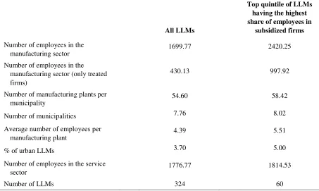
The overall results of this matching process are summarized in Table 1. On average, in the 324 LLMs
of the Mezzogiorno,11 there were approximately 1.7 thousand employees in manufacturing and 1.8
thousand employees in other sectors, excluding sectors not covered by the INPS archives (i.e.,
agriculture, public administration (PA) and self-employment) in 1995. On average, 25.3% of the
employees in the manufacturing sector worked in a subsidized firm. This percentage rose to 41.2%
in the top quintile of LLMs, having the highest share of employees in subsidized firms. The average
number of employees in manufacturing was 4.4, confirming the large proportion of micro and small
businesses in the Mezzogiorno, while the average number of firms per LLM was 54.6.
Insert Table 1
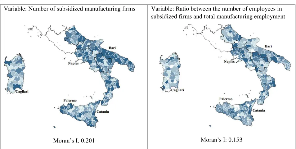
Figure 1 shows the geographic distribution of the intervention, displaying the number of employees
in subsidized firms per LLM in 2006, the final year of our sample. Almost all LLMs contain
subsidized firms, which were more predominant in Campania, in the eastern LLMs and in the coastal
areas of Sardinia and Sicily.
Insert Figure 1
11 In the Mezzogiorno, there are 325 LLMs, but we exclude the LLM of Naples as it is an outlier. In fact, it is the only
In Figure 2, we show the evolution of employment in the manufacturing sector for all firms, for the
subsidized ones and for the employment level forecasted by the entrepreneur (our instrument). The
maps show that there is a positive relationship between subsidy intensity and employment change
and that there is a significant overlap between expected and actual employment. If we consider this
as the ‘first stage’ of an IV regression, where forecasted employment in manufacturing predicts actual
employment in manufacturing, we obtain a F-statistic equal to 15.9, a R-squared of 0.47 and a
t-statistic for the main coefficient of 4.0. Moreover, in all the maps, we use the Moran’s I index to test
for the existence of spatial autocorrelation. The index is always positive, even if with a limited
magnitude, signaling the possible presence of spatial interactions among LLMs. Hence, we will take
spatial effects into account in the second part of the empirical analysis.
Insert Figure 2
6. Empirical analysis
The empirical analysis is based on the model proposed by Moretti and Thulin (2013) in its extended
version, described in equations (3) and (4). In equation (3), the shock variable is the absolute change
in employment in the tradable sector in the period 1995 to 2006, and the dependent variable is the
absolute change in employment in the service sector (such as approximation of non-tradable,
excluding PA-related sectors such as education, as well as to the entire PA sector). Likewise, in
equation (4), the shock variable is the absolute change in employment in the subsidized tradable sector
in the period 1995 to 2006, and the dependent variable is the absolute change in employment in the
non-subsidized tradable sector. Both models are then extended by conditioning on covariates that
take into account the characteristics of the business environment, such as the average firm size
(manufacturing and not), the concentration of firms by municipality (manufacturing and not), the
LLM surface area, the presence of urban areas and the pretreatment trend. Finally, regional fixed
In this section, the main focus is the IV estimates, even if we report also the OLS estimates. The local
multiplier estimates for the non-tradable sector are presented in Table 2, while Table 3 reports the
local multipliers for the non-subsidized tradable sector. For each analysis, we present the results with
only the shock variable as independent variable (columns 1 and 5), with the addition of the
characteristics of the business environment (columns 2 and 6), with the addition of regional
fixed-effects (columns 3 and 7), and with the addition of pretreatment trends (columns 4 and 8).
Insert Tables 2 and 3
Concerning the estimates on the non-tradable sector, the multiplier is always positive, significantly
different from zero and not negligible. The addition of controls and the regional fixed-effects
substantially reduce the extent of the estimates, showing the presence of some type of endogeneity
corrected by fixed effects and covariates. This is clearer in the fully specified IV model, where
controlling for the pretreatment trend further reduces the size of the multiplier 𝑀. However, even
after adding all the controls, the size of the local multiplier is statistically significant at the 1% level
and economically large: every new place generated in manufacturing generates approximately 1.16
jobs in the tertiary sector. The results are compatible with the model proposed by Moretti (2010) and
Moretti and Thulin (2013), where the increase in income and well-being related to new jobs in
manufacturing sectors increases the activity (and employment) in the local non-tradable sectors.
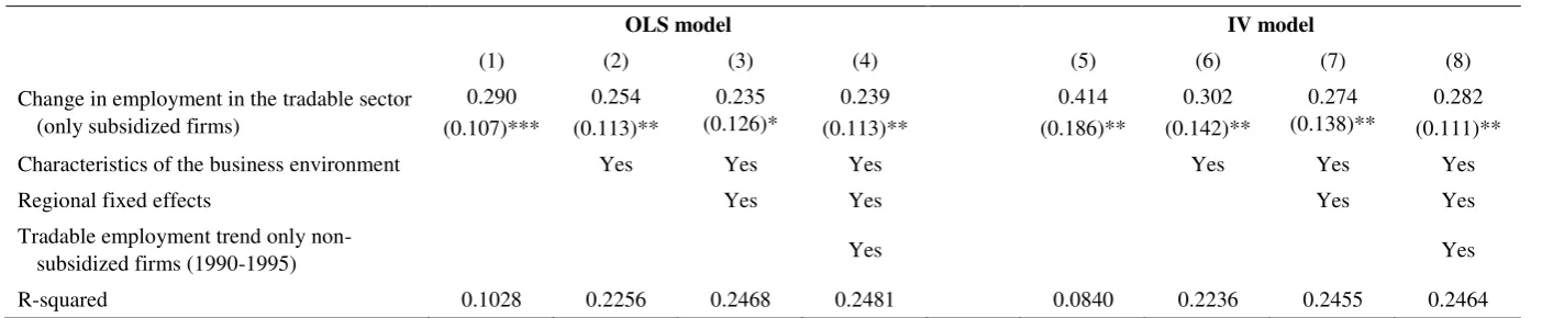
When we look at the relationship between the subsidized and the non-subsidized tradable sector, we
find once again that the local multiplier 𝑀′ is always positive and significantly different from zero at
the 5% level in all model specifications. The addition of controls, the regional fixed-effects and the
pretreatment trend reduce the extent of the estimates. This result is in line with the result for
non-tradable sectors. In the fully specified IV model, the local multiplier is 0.28, i.e., for every hundred
manufacturing firms. Therefore, in line with Moretti (2010), we find that the additional effects on
non-subsidized employment in manufacturing are limited but not negligible.
Following Duranton et al. (2011), we complement the empirical analysis combining spatial
differencing with instrumenting. This means that we apply the spatial difference operator, which takes
the difference between each LLM and any other bordering LLM, to equations (3) and (4), and then
we instrument the independent variable of interest. Spatial differencing conditions out LLM
unobserved heterogeneity; thereby, it is expected to reinforce the plausibility of the exclusion
restriction. The estimates reported in Table 4 are positive, statistically significant, very close to those
reported in Tables 2 and 3 and can be considered as a robustness analysis of the IV model.
Insert Table 4
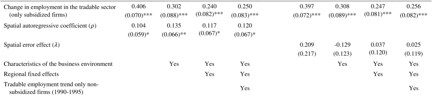
Finally, although spatial differencing takes into account spatial relations among neighboring LLMs,
it does not allow for estimating spatial spillovers.12 In Appendix A, we describe the potential channels
through which place-based policies could engender spillovers and the spatial models adopted to
estimate them. Table A1 of Appendix A reports the estimates obtained combining IV with the spatial
models. When we add spatial effects to the IV model, we obtain slightly lower local multiplier
estimates and spatial spillovers estimates that are rather small. However, it emerges that spillovers’
net impact is positive and statistically significant at the 10% level when we look at the relationship
between the subsidized and the non-subsidized tradable sector. This means that the tradable
employment growth in an LLM positively affects the employment growth in its neighboring LLMs,
signaling the possible presence of localization economies.
12 Gerolimetto and Magrini (2016) analyze a subset of US Metropolitan Statistical Areas to investigate to what extent
7. Concluding remarks: a comparison with the previous literature
In this paper, the employment multiplier of a large place-based policy in Southern Italy was computed
with a novel approach that exploits as instrument the entrepreneurs’ forecasts on employment linked
to subsidized projects. The multiplier linked to an occupational shock on the rest of the manufacturing
industry and the service sector is positively statistically significant and, particularly in the case of
services, economically large. Overall, an additional workplace in financed firms engenders the
creation of approximately 0.25-0.33 jobs in non-financed manufacturing firms and 0.93-1.16 jobs in
the service sector.
As shown in Table 5, these multipliers are only slightly lower than those found by Moretti (2010) and
van Dijk (2017) for US cities. Still, they are much higher than those previously documented for some
European countries, such as Italy, Spain and Sweden, and for Asian countries. There are many reasons
behind these differences. First, the use of comprehensive and accurate employment data derived from
the INPS archive has minimized the extent of the measurement error. Second, the use of a credible
instrument, which identifies the exogenous employment shock at the firm-level before the realization
of the incentivized project without being influenced by external shocks to the LLM economy, has
improved the identification of the local multipliers. Moreover, the local multipliers are derived from
the action of a real place-based policy and not by a hypothetical identification of local effects of a
nation-wide shock, increasing the external validity of the results.
Insert Table 5
Our interpretation of the high multipliers is mainly based on the presence of a large underutilization
of productive factors in the areas where L488 acted. We expect that where local unemployment is
high, local labor demand is very elastic, crowding out effects are low and the increase in local labor
cost are negligible (Moretti, 2010). This is the picture of the LLMs in the South of Italy, as they suffer
regions or abroad, while unskilled workers are more tied to local markets (Iuzzolino et al. 2013).
Therefore, the large multipliers are the effect of a very flexible local labor supply, which makes the
local economy more responsive to exogenous shocks, together with the efficiency of public spending
related to the L488 allocation procedure (see Cerqua and Pellegrini, 2014).
The main implication of our findings is that well-structured, efficient and well-managed place-based
policies, such as L488, have a positive and significant impact on local development, with large
employment multipliers. This increase is only partly offset by the presence of modest and negative
spillovers with adjacent areas, probably linked to rising labor costs and urban income. Additionally,
the effect is much larger in the non-tradable sector. This is consistent with Moretti's income effect,
which leads to redistribution of jobs between tradable and non-tradable sectors, coupled with the
Baumol’s disease (see Baumol, 1967), where the productivity growth gaps in the two sectors increase
the share of employment in the tertiary sector, as evidenced in developed countries.
Acknowledgments:This research has received support from the ‘VisitInps Scholars’ program. The
authors would like to thank Tito Boeri, Pietro Garibaldi, Massimo Antichi, Maria Domenica
Carnevale, Maria Cozzolino and Elio Bellucci for making INPS microdata available. We also
gratefully acknowledge helpful comments from participants at the VisitInps seminar, the Sapienza
DISSE seminar, and the Italian Regional Science Association 2017 conference.
References
Andini, M., de Blasio, G. (2016), Local development that money cannot buy: Italy’s Contratti di
Programma, Journal of Economic Geography, 16(2): 365–393.
Anselin, L. (1988), Spatial econometrics: methods and models, Kluwer Academic Publishers,
Bartik, T.J. (1991), Who benefits from state and local economic development policies? W.E. Upjohn
Institute for Employment Research.
Baum-Snow, N., Ferreira, F. (2015), Causal inference in urban and regional economics. In G.
Duranton, V. Henderson, & W. Strange (Eds.), Handbook of urban and regional economics 5 (pp. 3–
68), Amsterdam: Elsevier.
Baumol, W.J. (1967), Macroeconomics of unbalanced growth: The anatomy of urban crisis,
American Economic Review, 57(3): 415–426.
Becker, S.O., Egger, P.H., von Ehrlich, M. (2013), Absorptive capacity and the growth and
investment effects of regional transfers: A regression discontinuity design with heterogeneous
treatment effects, American Economic Journal: Economic Policy, 5(4): 29–77.
Belotti, F., Di Porto, E., Santoni, G. (2018), Spatial differencing: Estimation and inference. CESifo
Economic Studies, published online: 28 February 2018.
Blanchard, O.J., Katz, L.F. (1992), Regional Evolutions, Brookings Papers on Economic Activity
1992 (1): 1–75.
Cerqua, A., Pellegrini, G. (2014), Do subsidies to private capital boost firms' growth? A multiple
regression discontinuity design approach, Journal of Public Economics, 109: 114–126.
Cerqua, A., Pellegrini, G. (2017a), Are we spending too much to grow? The case of Structural Funds,
Journal of Regional Science, published online: 26 October 2017.
Cerqua, A., Pellegrini, G. (2017b), Industrial policy evaluation in the presence of spillovers, Small
Business Economics, 49(3): 671–686.
Cerqua, A., Pellegrini, G. (2018), Spatial mobility effects of a place-based policy, mimeo, Sapienza
University of Rome.
Chodorow-Reich, G., Feiveson, L., Liscow, Z., Gui Woolston, W. (2012), Does state fiscal relief
during recessions increase employment? Evidence from the American Recovery and Reinvestment
Act, American Economic Journal: Economic Policy, 4(3): 118–145.
Chodorow-Reich, G. (2017), Geographic cross-sectional fiscal spending multipliers: what have we
learned?, NBER Working Paper No. 23577.
Criscuolo, C., Martin, R., Overman, H. Van Reenen, J. (2018), Some causal effects of an industrial
policy, CEP Discussion Paper No. 1113 (Revised January 2018).
De Blasio, G., Menon, C. (2011), Local effects of manufacturing employment local effects of
De Castris, M., Pellegrini, G. (2012), Evaluation of spatial effects of capital subsidies in the South of
Italy, Regional Studies, 46(4): 525–538.
Drukker, D.M., Prucha, I.R., Raciborksi, R. (2013), A command for estimating spatial-autoregressive
models with spatial-autoregressive disturbances and additional endogenous variables, The Stata
Journal, 13: 287–301.
Duranton, G., Gobillon, L., Overman, H.G. (2011), Assessing the effects of local taxation using
microgeographic data, The Economic Journal, 121(555): 1017–1046.
Elhorst, J.P. (2010), Spatial panel data models. In M.M. Fischer & A. Getis (Eds.), Handbook of
applied spatial analysis (pp. 377–407), Heidelberg, Germany: Springer.
Einiö, E., Overman, H. (2016), The (displacement) effects of spatially targeted enterprise initiatives:
evidence from UK LEGI, CEPR Discussion Papers No. 11112.
Faggio, G., Overman, H. (2014), The effect of public sector employment on local labour markets.
Journal of Urban Economics, 79: 91–107.
Gerolimetto, M., Magrini, S. (2014), Spatial analysis of employment multipliers in Spanish labor
markets, Rivista Italiana di Economia Demografia e Statistica, LXVIII(3/4): 87–94.
Gerolimetto, M., Magrini, S. (2016), A spatial analysis of employment multipliers in the US, Letters
in Spatial and Resource Sciences, 9: 277–285.
Glaeser, E.L. (2001), The economics of location-based tax incentives, Discussion Paper No. 1932,
Harvard Institute of Economic Research, Harvard, MA.
Goldsmith-Pinkham, P., Sorkin, I., Swift, H. (2017), Bartik instruments: what, when, why and how,
mimeo, July 2017 version.
Kazekami, S. (2017), Local multipliers, mobility, and agglomeration economies, Industrial Relations,
56(3): 489–513.
Iuzzolino, G., Pellegrini, G., Viesti, G. (2013), Regional convergence, in G. Toniolo (editor), The
Oxford Handbook of the Italian Economy Since Unification, Oxford University Press.
LeSage, J.P. (2014), What regional scientists need to know about spatial econometrics, The Review
of Regional Studies, 44: 13–32.
Moretti, E. (2010), Local multipliers, American Economic Review: Papers and Proceedings, 100: 1–
Moretti, E., Thulin, P. (2013), Local multipliers and human capital in the United States and Sweden,
Industrial and Corporate Change, 22(1): 339–362.
Nakamura, E., Steinsson, J. (2014), Fiscal stimulus in a monetary union: evidence from US regions,
American Economic Review, 104: 753–792.
Serrato Suarez, J.C., Wingender, P. (2016), Estimating local fiscal multipliers, NBER Working
Paper No. 22425.
Shoag, D. (2013), Using state pension shocks to estimate fiscal multipliers since the Great Recession,
American Economic Review: Papers & Proceedings, 103: 121–124.
Van Dijk, H.J. (2017), Local employment multipliers in U.S. cities, Journal of Economic Geography,
17: 465–487.
Wang, T., Chanda, A. (2017), Manufacturing growth and local multipliers in China, Journal of
Comparative Economics, advance online publication: 28 October 2017.
Wilson, D.J. (2012), Fiscal spending job multipliers: evidence from the 2009 American Recovery
Appendix A – The combination of IV with spatial models
IV estimation can be combined with a spatial model. We adopt the spatial model to take into account
the presence of clusters of neighboring LLMs sharing high or low rates of employment variables (as
the maps in Figures 1 and 2 show), which give rise to spatial dependence or spatial autocorrelation
(Anselin, 1988). When specifying the interactions between spatial units, the model may contain a
spatially lagged dependent variable or a spatial autoregressive process in the error term, known as the
spatial autoregressive model (SAR) reported in equation (5) and the spatial error model (SEM)
reported in equation (6), respectively (Elhorst, 2010)13:
(1 − ρ𝐖) ∗ Δ𝐸𝑙𝑁𝑇= 𝛼 + 𝜃Δ𝐸𝑙𝑇+ β𝐗𝑙+ Δ𝐸𝑙,𝑡−1𝑁𝑇 + v + 𝜀𝑙 (5)
{Δ𝐸𝑙𝑁𝑇= 𝛼 + 𝜃Δ𝐸(1 − λ𝐖) ∗ 𝜙𝑙𝑇+ β𝐗𝑙+ Δ𝐸𝑙,𝑡−1𝑁𝑇 + v + 𝜙𝑙
𝑙 = 𝜀𝑙
(6)
where W represents the row-standardized spatial contiguity matrix that assigns a positive value only
to neighboring LLMs (rook contiguity), 𝜌 reflects the spatial autoregressive coefficient, 𝜙𝑙 reflects
the spatially autocorrelated error term and 𝜆 reflects the spatial autocorrelation coefficient. The
spatial models are based on two different assumptions: SAR posits that the dependent variable
depends on the dependent variable observed in neighboring LLMs and on a set of observed local
characteristics, while SEM posits that neighbors are subject to correlated random shocks, which
determine a correlation between LLMs’ employment outcomes, which could be erroneously
interpreted as causal influence. Spatial models are estimated using a spatial two-step least squares
approach through the Stata command ‘spivreg’ (Drukker et. al. 2013). We use these models to test
whether spillover effects are in place, i.e., if the change in employment in LLM 𝑙 is not only
determined by its own local conditions but also affected by the change in the employment level of
neighboring LLMs. The linkage between neighboring LLMs that generates spatial spillovers is
curiously little considered in the literature, although incentive policies for businesses, particularly
those aimed at the growth of less developed regional areas, are designed to promote local business
aggregations in the area, producing local agglomerations that generate spatial externalities or positive
spillovers (De Castris and Pellegrini, 2012).
Place-based policies might engender positive externalities on the supply and demand of goods and
services in two ways: i) generating income that converts into local taxes that then fall into the form
of public expenditure on the territory and ii) subsidizing the construction of fixed assets in the area
which ultimately have a positive impact on public and private income (see Glaeser, 2001). However,
subsidized firms could displace businesses and investments in neighboring areas, with a spatial
crowding-out effect on production and labor markets. These conflicting hypotheses make it difficult
to assess the theoretical net effect of spillovers, leaving to the empirical analysis the task of
determining it.
Looking at the spatial model estimates reported in Table A1, it emerges that spillovers net impact is
positive, that is, the employment growth in an LLM has a positive impact on the employment growth
in its neighboring LLMs. However, it emerges that spillover net impact is statistically significant at
the 10% level only when we look at the relationship between the subsidized and the non-subsidized
tradable sector, yet when we add spatial effects to the IV model, we obtain slightly lower local
multiplier estimates, namely, a multiplier of 0.26 for the non-subsidized tradable sector and of 0.93
for the non-tradable sector. Following LeSage (2014), we also estimated the spatial Durbin error
model (SDEM), which contains the spatially lagged independent variables and a spatial
autoregressive process in the error term. Using SDEM we get estimates similar to those obtained
using SEM.
Table 1 – Descriptive statistics
All LLMs
Top quintile of LLMs having the highest share of employees in
subsidized firms Number of employees in the
manufacturing sector
1699.77 2420.25
Number of employees in the manufacturing sector (only treated firms)
430.13 997.92
Number of manufacturing plants per municipality
54.60 58.42
Number of municipalities 7.76 8.02
Average number of employees per manufacturing plant
4.39 5.51
% of urban LLMs 3.70 5.00
Number of employees in the service sector
1776.77 1814.53
Number of LLMs 324 60
Table 2 - Local multipliers for the non-tradable sector
Dependent variable: Change in employment in the service sector
OLS model IV model
(1) (2) (3) (4) (5) (6) (7) (8)
Change in employment in the tradable sector 2.483 (0.408)***
0.327 (0.074)***
0.280 (0.076)***
0.616 (0.174)***
6.480 (1.588)***
1.809 (0.672)***
1.829 (0.702)***
1.164 (0.367)*** Characteristics of the business environment Yes Yes Yes Yes Yes Yes
Regional fixed effects Yes Yes Yes Yes
Non-tradable employment trend (1990-1995) Yes Yes
R-squared 0.1872 0.7374 0.7416 0.9267 N/A 0.6878 0.6894 0.9202
Notes: All Southern LLMs are included in the analysis with the exception of Naples for a total of 324 observations. Standard errors are clustered at the regional level. The control variables are: the average size of local firms (manufacturing and service sectors), the concentration of plants per municipality (manufacturing and service sectors), the surface area of the LLM and a dummy equal to one for LLM containing an urban area.
Table 3 - Local multipliers for the tradable sector
Dependent variable: Change in employment in the manufacturing sector (only non-subsidized firms)
OLS model IV model
(1) (2) (3) (4) (5) (6) (7) (8)
Change in employment in the tradable sector (only subsidized firms)
0.290 (0.107)***
0.254 (0.113)**
0.235 (0.126)*
0.239 (0.113)**
0.414 (0.186)**
0.302 (0.142)**
0.274 (0.138)**
0.282 (0.111)** Characteristics of the business environment Yes Yes Yes Yes Yes Yes
Regional fixed effects Yes Yes Yes Yes
Tradable employment trend only
non-subsidized firms (1990-1995) Yes Yes
R-squared 0.1028 0.2256 0.2468 0.2481 0.0840 0.2236 0.2455 0.2464 Notes: All Southern LLMs are included in the analysis with the exception of Naples for a total of 324 observations. Standard errors are clustered at the regional level. The control variables are: the average size of local manufacturing firms, the concentration of manufacturing plants per municipality, the surface area of the LLM and a dummy equal to one for LLM containing an urban area.
Table 4 - Local multipliers for the non-tradable and tradable sectors combining IV with spatial differencing
Dependent variable: Change in employment in the service sector
(1) (2) (3) (4)
Change in employment in the tradable sector 7.228 (1.444)*** 1.197 (0.719) 1.260 (0.774) 1.078 (0.596)* Characteristics of the business environment Yes Yes Yes
Regional fixed effects Yes Yes
Non-tradable employment trend (1990-1995) Yes
Dependent variable: Change in employment in the manufacturing sector (only non-subsidized firms)
Change in employment in the tradable sector (only subsidized firms)
0.383 (0.175)** 0.341 (0.094)*** 0.318 (0.090)*** 0.329 (0.091)*** Characteristics of the business environment Yes Yes Yes
Regional fixed effects Yes Yes
Tradable employment trend only
non-subsidized firms (1990-1995) Yes
Notes: All Southern LLMs are included in the analysis with the exception of Naples for a total of 324 observations. Standard errors are clustered at the regional level. These models have been estimated through the Stata command sreg developed by Belotti et al. (2018). The control variables are: the average size of local firms (manufacturing and service sectors), the concentration of plants per municipality (manufacturing and service sectors), the surface area of the LLM and a dummy equal to one for LLM containing an urban area in the top panel, and the average size of local manufacturing firms, the concentration of manufacturing plants per municipality, the surface area of the LLM and a dummy equal to one for LLM containing an urban area in the bottom panel.
Table 5 – Estimates of local multipliers: comparison among papers
Local multiplier – tradable sector
Local multiplier –
non-tradable sector Area Method
Our paper
0.28 (0.14)* 1.16 (0.37)*** Mezzogiorno LLMs Instrument: forecasted employment in L488
0.33 (0.09)*** 1.08 (0.60)* Mezzogiorno LLMs Instrument: forecasted employment in L488. IV with spatial differencing
Moretti (2010) 0.26 (0.23) 1.59 (0.26)*** U.S. metropolitan cities Bartik instrument
Van Dijk (2017) N/A 1.58 (0.31)*** U.S. metropolitan cities Bartik instrument
Moretti and Thulin (2013) 0.41 (0.15)*** 0.49 (0.29)* Sweden LLMs Bartik instrument: all tradable sector
Gerolimetto and Magrini (2014) N/A 0.04 (0.18) Spain LLMs Bartik instrument
De Blasio and Menon (2011)
-0.47 (0.71) -0.09 (0.10) Italy LLMs Bartik instrument
-0.17 (0.41) -0.15 (0.13) Mezzogiorno LLMs Bartik instrument
Kazekami (2017) N/A 0.41(0.25)* high mobility
0.09 (0.13) low mobility Japan commuting zones Bartik instrument
Wang and Chanda (2017) N/A 0.34 (0.14)** China prefecture-level
cities Bartik instrument
Table A1 - Local multipliers for the non-tradable and tradable sectors combining IV with spatial models
Dependent variable: Change in employment in the service sector
IV estimation of the spatial error model IV estimation of the spatial autoregressive model
(1) (2) (3) (4) (5) (6) (7) (8)
Change in employment in the tradable sector 6.492 (0.571)*** 1.622 (0.416)*** 1.412 (0.389)*** 1.009 (0.196)*** 6.546 (0.583)*** 1.636 (0.412)*** 1.286 (0.372)*** 0.931 (0.187)*** Spatial autoregressive coefficient (𝜌) -0.053
(0.040) 0.015 (0.047) -0.003 (0.049) 0.032 (0.067)
Spatial error effect (𝜆) -0.159
(0.098) -0.085 (0.042)** -0.065 (0.041) -0.009 (0.020) Characteristics of the business environment Yes Yes Yes Yes Yes Yes
Regional fixed effects Yes Yes Yes Yes
Non-tradable employment trend (1990-1995) Yes Yes
Dependent variable: Change in employment in the manufacturing sector (only non-subsidized firms)
Change in employment in the tradable sector (only subsidized firms)
0.406 (0.070)*** 0.302 (0.088)*** 0.240 (0.082)*** 0.250 (0.083)*** 0.397 (0.072)*** 0.308 (0.089)*** 0.247 (0.081)*** 0.256 (0.082)*** Spatial autoregressive coefficient (𝜌) 0.104
(0.059)* 0.135 (0.066)** 0.117 (0.067)* 0.120 (0.067)*
Spatial error effect (𝜆) 0.209
(0.217) -0.129 (0.123) 0.037 (0.120) 0.025 (0.119) Characteristics of the business environment Yes Yes Yes Yes Yes Yes
Regional fixed effects Yes Yes Yes Yes
Tradable employment trend only
non-subsidized firms (1990-1995) Yes Yes
Notes: All Southern LLMs are included in the analysis with the exception of Naples for a total of 324 observations. We employ the rook contiguity spatial matrix to estimate the spatial models. These models have been estimated through the Stata command spivreg. The control variables are: the average size of local firms (manufacturing and service sectors), the concentration of plants per municipality (manufacturing and service sectors), the surface area of the LLM and a dummy equal to one for LLM containing an urban area in the top panel, and the average size of local manufacturing firms, the concentration of manufacturing plants per municipality, the surface area of the LLM and a dummy equal to one for LLM containing an urban area in the bottom panel.
Figure 1 – Spatial distribution of employment variables in 2006
Variable: Number of subsidized manufacturing firms
Moran’s I: 0.201
Variable: Ratio between the number of employees in subsidized firms and total manufacturing employment
Moran’s I: 0.153
35 Figure 2 – Spatial distribution of manufacturing employment change over the period 1995-2006.
Variable: Employment growth rate in manufacturing
Moran’s I: 0.078
Variable: Employment growth rate in manufacturing (only subsidized firms)
Moran’s I: 0.050
Variable: Forecasted employment growth rate in subsidized manufacturing firms
Moran’s I: 0.133