North South Trade and Uneven Development in a Classical Conventional Wage Share Growth Model

Munich Personal RePEc Archive

North-South Trade and Uneven

Development in a Classical Conventional

Wage Share Growth Model

Sasaki, Hiroaki

24 August 2018

Online at

https://mpra.ub.uni-muenchen.de/88631/

North-South Trade and Uneven Development in a

Classical Conventional Wage Share Growth Model

Hiroaki SASAKI

August 2018

Abstract

This study presents a model of North-South trade and uneven development, and inves-tigates the growth rates of both countries under the trade pattern such that the North

specializes in investment goods while the South specializes in consumption goods. In contrast to existing studies, we close the model by fixing each countries’ income dis-tribution, specifically, the ratio of labor share to capital share. Using the model, we

conduct the following two analyses. First, assuming that both countries already en-gage in international trade and that the North specializes in investment goods while the South specializes in consumption goods, we investigate the dynamics of both countries’

growth rates and the terms of trade. Second, we investigate the condition under which such a trade pattern holds, and compare equilibrium variables under autarky and

equi-librium values under free trade. From the first analysis, it follows that both countries grow at the same rate in the long run. From the second analysis, however, it follows that in the first place, the terms of trade must lie within the interval between the relative

prices of both countries and that both countries’ growth rates may not equalize as long as both countries engage in trade.

Keywords: North-South trade; Uneven development; Conventional wage share; Com-parative advantage

JEL Classification: F10; F43; O33; O41

1

Introduction

This study presents a two-country, two-good, two-factor growth model, and investigates the growth rates of two countries in a North-South framework. As many existing studies

show, one can build a variety of models depending on the “closures” of models: what is the closure of the model? For example, in the Heckscher-Ohlin-Samuelson model and the dynamic version of the Heckscher-Ohlin-Samuelson model, full-employment of labor and full-utilization of capital are imposed to close the model. If the labor market of the North is tightened and the labor market of the South faces surplus of labor, we can impose a full-employment of labor condition on the North while we can impose a fixed real wage rate on the South. If in the North, the wage rate is determined by labor-management bargaining while in the South, the labor market faces surplus of labor, we can close the model by setting both counters’ real wage rates constant.

A pioneering study that investigates the relationship between North-South trade and eco-nomic growth is Findlay (1980). He assumes that the North is a Solow-type economy while the South is a Lewis-type economy. That is, to close the model, he imposes full-employment of labor and full-utilization of capital conditions on the North and imposes fixed real wage rate on the South. The result shows that in the long run, the terms of trade is constant and both countries grow at the same rate. He assumes that both countries are engaged in free trade from the start and that the North exports manufacturing goods while the South exports agricultural goods.

After Findlay (1981), many studies of North-South trade and economic growth are pro-duced (Taylor, 1981; Molana and Vines, 1989; Sarkar, 2001; Dutt, 1996, 2002; Chui, et al., 2002). However, these existing studies fix trade patterns and investigate a situation where both countries engage in international trade from the start.1 _{For this reason, they cannot}

compare a situation under autarky and a situation under free trade.

As studies that compares a situation under autarky and a situation after trade in a North-South framework, we can take Mainwaring (1974) and Ho (1997).2 _{Mainwaring (1974)}

assumes that the profit rate is constant both under autarky and free trade to close the model, and compares the long-run equilibrium under autarky and that under free trade. Ho (1997) considers a situation where the North has an absolute advantage over the South, that is, every input coefficient of the North is less than each corresponding input coefficient of the South, and the North has a comparative advantage in investment goods while the South has a comparative advantage in consumption goods. Then, he examines how both countries growth rates evolve after trade. He assumes that the real wage rates of both countries are constant before and after trade.

We also provide a model of North-South trade and economic growth. In our analysis, based on the idea of modern classical economics such as Foley and Michl (1999), we close

1_{For studies that consider North-South trade and economic growth, see also Blecker (1996), Conway and} Darity (1991), Darity (1990), Dutt (1988), Sarkar (1989, 1997), and Sasaki (2011a).

the model with the assumption that income distribution (labor share and capital share) of each country is constant before and after trade. The fact that long-run income distribu-tion is constant in many countries is well known, and hence, the assumpdistribu-tion of constant labor/capital share is reasonable.

Using the model, we consider two cases. First, under the assumption the both countries engage in free trade from the start and that the North specializes in investment goods while the South specializes in the consumption goods, we investigate the dynamics of the terms of trade and growth rates of both countries. Second, we derive the condition under which such a trade pattern emerges, and compare each variable under autarky and the corresponding variable under free trade. From the first analysis, we can show that the terms of trade be-comes constant and both countries growth at the same rate in the long run. From the second analysis, we can show that for both countries to engage in free trade, the terms of trade must lie within the interval between the relative price of the North and that of the South under autarky, and that both countries can grow at different rates as long as both countries engage in trade. In other words, the result from the analysis that ignores comparative advantage and the result from the analysis that considers comparative advantage are different.

Our model is based on the classical conventional wage share model presented by Foley and Michl (1999). Here, the conventional wage share means that labor share is exogenously given due to some institutional factors. They consider an economy in which both workers and capitalists coexist, workers consume all wage income, capitalists save a constant fraction of profit, and a single good is produced by a Leontief production function. Then, they investigate the economic growth rate and show that the economic growth rate is increasing in both the saving rate of capitalists and capital share. We extend the Foley-Michl model to a two-country, two-good model, and investigate international trade between two countries.

The idea of the present paper is based on the idea of above-mentioned Ho (1997). He presents a classical growth model that investigates the relationship between North-South trade and growth. In his analysis, he fixes both countries’ real wage rates to close the model. Since the real wage rates in both countries are constant before and after trade, the welfare of workers in terms of real wage is constant before and after trade. In contrast, in our model, the real wage rates in both countries can change before and after trade. Therefore, our model can capture a change in welfare by international trade.

We assume that the North has a comparative advantage in investment goods while the South has a comparative advantage in consumption goods. Then, we examine how both countries’ growth rates change when switching from autarky to free trade. Section 6 concludes.

2

Autarky

Suppose an economy in which both workers and capitalists coexist. Workers earn wage income by labor, consume all the wage income, and hence, do not save. Capitalists earn profit by lending capital, save a constant proportion of the profit. In this economy, there are investment goods and consumption goods. We assume that investment goods are dedicated for investment while consumption goods are dedicated for consumption. Let the investment goods sector and the consumption goods sector be sector 1 and sector 2, respectively. Let the output of sector 1 and that of sector 2 beIandC, respectively. Production of both goods requires labor and capital. We assume that each production function takes the following Leontief production function.

I =min_{(1/v1)N1,(1/h1)K1}, (1)

C =min_{(1/v2)N2,(1/h2)K2}, (2)

whereNi denotes the employment of sector i; Ki, the capital stock of sectori;vi, the labor

input coefficient of sectori; andhi, the capital coefficient of sectori.

Suppose the total employment is N = N1 +N2, total capital stock isK = K1+ K2, the

relative price of investment goods in terms of consumption goods is p, the real wage rate is

ω, and the profit rate isr. Then, the equilibrium under autarky is described by the following six equations.

v1I+v2C =N, (3)

h1I+h2C =K, (4)

p= v1ω+ ph1r, (5)

1=v2ω+ph2r, (6)

I= srK, 0< s<1, (7)

ωN

r pK =θ, θ >1. (8)

goods and consumption goods. Equation (5) shows the price equation of investment goods and equation (6) shows the price equation of consumption goods. Equation (7) shows equi-librium of goods market, that is, investment is equal to saving. Equation (8) shows that the ratio of labor share to capital share is fixed asθ.3 _{We assume thatθ >1 because labor share}

is larger than capital share in reality. For six endogenous variablesI,C, N, p,ω, and r, we have six equations, and hence, the system is closed.

The equilibrium solutions of the system are given as follows:4

First, for price variables, we obtain

r_∗= [(1+s)m+θ−s]−

√

[(1+ s)m+θ₋s]2_{−4sm(m−1)}

2sh1(m−1)

, (9)

p_∗= v1

v2+(v1h2−v2h1)r∗

, (10)

ω_∗= 1−h1r∗

v2+(v1h2−v2h1)r∗

, (11)

wherem _≡(h1

v1)/(

h2

v2). An asterisk “*” denotes an equilibrium value. Appendix 2 shows that

∂r_∗/∂θ <0 and Appendix 3 shows that∂r_∗/∂m>0 whenh1is constant.

Second, for quantity variables, we obtain

I_∗= sr_∗K, (12)

N_∗= v1

h1

K, (13)

C_∗= ω_∗N_∗+(1₋ s)p_∗r_∗K. (14)

Note that these price and quantity variables exist for countries A and B. The economic growth rate is given byg_∗ = sr_∗.

3

Free Trade

Suppose that in the world economy, there are two countries: country A is the North and country B is the South. Suppose that from the start, both countries A and B engage in free trade and that country A specializes in investment goods while country B specializes in consumption goods. Let the world demand for investment and the world demand for consumption beIw andCw, respectively. Under this trade pattern, we obtain the following

3_{The specification of equation under autarky is based on Uni (1996) and Sasaki (2008).}

relationships.

Iw= 1

v₁A N

A ₌ 1

hA₁ K

A_{, (15)}

Cw= 1

vB

2

NB = 1

hB

2

KB. (16)

From equations (15) and (16), each country’s employment is given by

NA = v

A

1

hA

1

KA, (17)

NB = v

B

2

hB

2

KB. (18)

Equations for income distribution are given by

ωA T

pTrAT

vA

1

hA

1

=θA, (19)

ωB T

pTrB_T

v₂B hB

2

=θB. (20)

A variable “T” denotes free trade.

Price equations under free trade are given by

pT =vA1ω

A_{+ p} ThA1r

A

T, (21)

1=v₂BωB+ pThB2r

B

T. (22)

World saving and world investment are equalized, and then, we have

X₁A = K

A

hA

1

= sAr_TAKA+sBrB_TKB =_⇒ 1

hA

1

= sArA_T +sBr_TBκ, (23)

whereκ _≡ KB_/KA _{denotes the capital stock ratio. Each capital stock is given at some point}

in time. However, each capital stock evolves through time by investment.

There are five endogenous variables,pT,ωA_T,r_TA,ω_TB, andωB_T, and there are five equations

(19), (20), (21), (22), and (23). Therefore, we can solve for equilibrium prices. From these equilibrium price variables, we obtain equilibrium quantity variables.

First, for equilibrium price variables. we obtain

r_TA = 1

hA

1(1+θA)

r_TB = 1+θ

A

−sA sB_hA

1(1+θA)κ

, (25)

ωA_T = h

A

1

vA₁h₂B

θA

(1+θB₎

sB

(1+θA_{− s}A₎κ, (26)

ω_TB = 1

vB

2 θB

(1+θB₎, (27)

pT =

hA₁ h₂B

(1+θA₎

(1+θB₎

sB

(1+θA_−sA₎κ. (28)

The profit rate of country A and the real wage rate of country B do not depend on κ, and hence, these variables stay constant through time. In contrast, the profit rate of country B is a decreasing function ofκ, the real wage rate of country A is an increasing function ofκ, and hence, these variables change through time. The terms of trade is an increasing function of

κ.

Second, for equilibrium quantity variables, we obtain

I_TA = sAr_TAKA, (29)

I_TB = sBr_TBKB, (30)

N_TA = v

A

1

hA

1

KA, (31)

N_TB = v

B

2

hB

2

KB, (32)

C_TA =ωA_TN_TA+(1₋ sA)p_TAr_TAKA, (33)

C_TB =ωB_TN_TB+(1₋ sB)p_TBr_TBKB. (34)

4

Long-run dynamics

We investigate the dynamics of both countries’ growth ratesg_TA = sAr_TA andgB_T = sBr_TB with the assumption that country A specializes in investment goods and country B specializes in consumption goods. First, from equation (24), the profit rate of country A does not depend onκ, and hence,gA_T does not depend on time. In contrast, from equation (25), the profit rate of country B depends onκ, and henceg_TBalso depends onκ.

g_TB(t)= sBr_TB(t)= 1+θ

A_−sA

hA

1(1+θA)

1

The growth rate ofκ(t) is given by ˙κ(t)/κ(t)= gB T(t)−g

A

T, and hence, from equation (35), the

dynamics ofgB

T(t) is given by

˙

gB_T(t)=₋gB_T(t)[gB_T(t)₋gA_T]. (36)

At the steady state where ˙gB_T(t)=0, we haveg_TB(t)= g_TA. Sincedg˙B_T(t)/dg_TB(t)< 0, the steady state is stable. Then, at the steady state, we obtain

¯

g_TB =g¯_TA = s

A

hA

1(1+θA)

. (37)

A variables with a bar denotes a steady state value. FromgA

T = gBT, we have sArTA = sBrTB,

and hence, the capital stock ratio in the long run is given by

¯

κ= 1+θ

A_−sA

sA . (38)

Using equation (38), at the long-run equilibrium, we obtain the real wage rate of country A, the profit rate of country B, and the terms of trade as follows:

¯

ωA_T = h

A

1

vA

1hB2 θA

1+θB

sB

sA, (39)

¯

r_TB= 1

hA

1

1 1+θA

sA sB

, (40)

¯

pT =

hA

1

hB₂

1+θA

1+θB

sB

sA. (41)

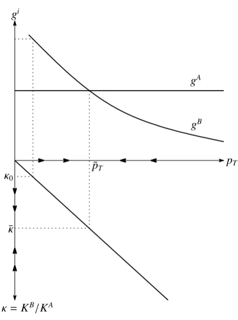
The above analysis can be also summarized by using Figure 1. At the first quadrant of Figure 1, the horizontal axis and the vertical axis denote the terms of trade and growth rates, respectively. The growth rate of country A is horizontal line. The growth rate of country B is a downward sloping curve. At the intersection of the two graphs, the terms of trade and the growth rates of both countries in the long-run equilibrium are determined. At the second quadrant of Figure 2, the vertical axis denotes the capital stock ratio. The graph of the second quadrant shows that the terms of trade is an increasing function of the capital stock ratio. As long as gA > gB, κ decrease and the terms of trade also decreases. When

gA = gB,κbecomes constant and the terms of trade also becomes constant. WhengA < gB,

gA

gB

pT

gi

κ= KB/KA

κ₀

¯

κ

¯

pT

Figure 1: Convergence to long-run equilibrium

5

Switch from autarky to free trade

In this section, we assume that counry A has an absolute advantage over coountry B and that country A has a comparative advantage in investment goods while country B has a comparative advantage in consumption goods, and investigate how each variable changes when the economy switches from autarky to free trade.

As we explain in the Introduction, similar analysis is conducted by Ho (1997). He as-sumes that the real wage rates of both countries are fixed and the same under autarky and free trade. Then, he shows that the gap betweengA _andgB _{under autarky can expand under}

free trade.

In contrast, we assume that income distribution of both countries are fixed and the same under autarky and free trade. Since the real wage rate can change after free trade starts, we will obtain a conclusion different from the conclusion of Ho (1997).

must lie within the interval of pA_{and p}B_{. He also assumes that country A has a comparative}

advantage in investment goods and country B has a comparative advantage in consumption goods, and hence, pA _{≤ p}

T ≤ pB must hold as long as both countries engaged in free trade.

Then, under his setting, the curve that shows the relationship between pT and gA and the

curve that shows the relationship between pT andgB do not intersect within the interval of

pA

≤ pT ≤ pB. Therefore, as long as both countries engage in free trade,gA = gB does not

hold.

Based on the method of Ho (1997), we examine how each variable changes when both countries switch from autarky to free trade. The problem is that it is difficult to use the graphical analysis. When the real wage rates are fixed like Ho (1997), the curve that shows the relationship between the terms of trade and the growth rate is uniquely determined in response to an arbitrary real wage rate. In our model, however, the real wage rate can change when both countries switch to free trade, and hence, we cannot easily draw the curve that shows the relationship between the terms of trade and the growth rate.

Fortunately, we can analytically obtain all the endogenous variables. Accordingly, by giving numerical values to the parameters, we can numerically compute all the endogenous variables. Note that we must condider the following issues.

1. All the input coefficients of country A are less than those of country B: country A has an absolute advantage over country B.

2. The terms of trade must lie within the interval between the relative price of country A and that of country B under autarky: country A has a comparative advantage in investment goods and country B has a comparative advantage in consumption goods.

3. The distributional parameterθand the saving rate sof country A are same as those of country B for ease of exposition.

By finding out combinations of the parameters that satisfy the above conditions, we calculate each variable under autarky and free trade.

We consider the following numerical example. First, suppose that the saving rates of capitalist are the same in both countries, sA _{= s}B _{= 0.5. Second, suppose that the}

distribu-tional parameters are also the same in both countries, θA _{= θ}B _{= θ = 1.375. Third, we set}

the input coefficients and the capital stock ratio as follows:

vA₁ = 1, vA₂ =2.4, hA₁ = 1, h₂A =1.6,

These examples satisfy the condition that country A has an absolute advantage in both sec-tors 1 and 2.

Table 1 shows our results. Under autarky, we have rA _{= 0.5, ω}A _{= 0.25, p}A _{= 0.5.}

rB _{= 0.314, ω}B _{= 0.127, and p}B _{= 0.684. The profit rate of country A exceeds that of}

country B. Since, pA _{< p}B_{, country A has a comparative advantage in investment goods}

while country B has a comparative advantage in consumption goods. After trade starts, the profit rates and the real wage rates arerA

T =0.421,ω A

T = 0.363,r B

T = 0.395, andω B

T = 0.116.

Then, by free trade, in country A, the profit rate decreases while the real wage rate increases. In contrast, in country B, the profit rate increases while the real wage rate decreases. The terms of trade is pT = 0.627, which lies within the interval of pA < pT < pB.

[Table 1 around here]

Under this setting, when both countries switch from autarky to free trade, we havegA >

gB. Thus, κ decreases through time. When gA = gB, the terms of trade is given by ¯pT =

0.588, which lies within the interval between pA and pB. Therefore, in the long run, both countries grow at the same rate.

Next, we change only hB₂ from hB₂ = 1.7 to hB₂ = 2.1. The results are given in Table 2. We have pA = 0.5, pB = 0.608, and pT = 0.508, and hence, country A has a comparative

advantage in investment goods while country B has a comparative advantage in consumption goods. The terms of trade such that gA = gB is given by ¯pT = 0.476, which does not

lie within the interval of pA < pT < pB. Accordingly, the terms of trade ¯pT = 0.476 is

infeasible. Therefore, both countries’ growth rates are not the same in the long run. In this case, we have pT = pA in the long run. Then, we can computeκ such that pT = pA.

Substituting the resultantκ= 3.94 into g_TB = sBr_TB, we can obtain the growth rate of country B, which leads to gB_T = 0.201. From this, it follows that gA_T > gB_T, and therefore, both countries’ growth rates are not equalized.

[Table 2 around here]

6

Concluding remarks

assuming that from the start, the North specializes in investment goods while the South spe-cializes in consumption goods, we have investigated the dynamics of both countries’ growth rates and the terms of trade. Second, we have considered the condition under which such a trade pattern holds, and compared the equilibrium under autarky and that under free trade.

From the first investigation, we have shown that both countries grow at the same rate in the long run. From the second investigation, however, we have shown that the terms of trade must lie within the interval between the relative price of the North and that of the South under autarky and that both countries’ growth rates may not be equalized as long as both countries engage in free trade.

Many studies in this field assume that both countries engage in free trade from the start, and then, show that both countries’ growth rates are equalized. In contrast, by considering comparative advantage, we have shown that both countries’ growth rates may not be equal-ized. This suggests that if two countries that have different levels of technologies engage in free trade, the growth rates may not be equalized potentially.

Appendix 1

The profit rate in our system is two possible solutions of the following quadratic equation:

sh1(m−1)r2−[(1+ s)m+(θ−s)]r+

m h1

= 0. (42)

Whenm , _{1, we obtain two rs from equation (42).}5 _{However, one r does not fall within}

0<r< 1/h1, where 1/h1 is the maximum profit rate with the real wage rateω= 0.

Appendix 2

The partial derivative of the profit rate with respect to the distributional parameterθis cal-culated as follows:

∂r

∂θ =

1₋[(1+ s)m+θ₋s]{[(1+s)m+θ₋s]2_{−4sm(m−1)}}−

1 2

2sh1(m−1)

. (43)

We pay attention to the numerator. DefineA_≡ [(1+ s)m+θ₋s]>0. Acan be rewritten as

A=m+(m₋1)s+θ. Since 0 < s<1,m> 0, andθ >0, Ais necessarily greater than zero.

Then, the numerator becomes

1₋A[A2₋4sm(m₋1)]−12 =1−

√

A2

√

A2_{−4sm(m−1)}. (44)

Ifm>1, then √A2_> √_A2_{−4sm(m−1), and hence, we have}

1₋

√

A2

√

A2_{−4sm(m−1)} < 0. (45)

Therefore, since the numerator of the right-hand side of equation (43) is negative and the denominator is positive, we have∂r/∂θ <0.

If 0< m<1, then √A2 _< √_A2_{−4sm(m−1). Thus, we have}

1₋

√

A2

√

A2_{−4sm(m−1)}

> 0, (46)

so that the numerator of the right-hand side of equation (43) is positive and the denominator is negative. Thus, we obtain∂r/∂θ <0.

Ifm = 1, then we obtainr = 1/[h1(1+θ)] from equation (42). This clearly shows that ∂r/∂θ <0.

It follows from these that in every case an increase inθalways leads to a decline in the profit rate, other things being constant.

Appendix 3

The partial derivative of the profit rate with respect tomis calculated as follows. We have

∂A/∂m= 1+s. LetD_≡ √A2_{−4sm(m−1). Then, we have} ∂D

∂m = (A

2

−4sm2+4sm)−12[_A(1_+s)₋4_sm+2_s]. (47)

Moreover, we can rewriteras

r= 2

h1

( _m

A+D

)

| {z }

≡B

= 2

h1

B. (48)

From this, we have

∂r

∂m =

2

h1 ∂B

Accordingly, the sign of the partial derivative ofr with respect tom is equal to the sign of the partial derivative ofBwith respect tom. Then,

∂B

∂m =

(A+D)₋m(_∂∂_mA + ∂_∂D_m)

(A+D)2 . (50)

Since the denominator of equation (50) is positive, the sign of the right hand side of equation (50) is equal to the sign of the numerator. The numerator can be rewritten as

(A+D)₋m

(

∂A

∂m +

∂D

∂m

)

= AD+D

2

−m(1+ s)D₋mA(1+s)+4sm2₋2sm

D . (51)

Since the denominator of equation (51) is positive, we pay attention to the numerator of equation (51).

AD+D2₋m(1+ s)D₋mA(1+s)+4sm2₋2sm=(θ₋ s)(A+D)+2sm. (52)

From these, we obtain

∂r

∂m =

2

h1

(θ₋ s)(A+D)+2sm

D(A+D)2 . (53)

From economic data, the labor share in national income is larger than 1/2, which implies thatθ > 1. With A > 0,D > 0, and 0 < s < 1, the sign of equation (53) is always positive. Therefore, other things being equal, an increase in m always increases r as long as h1 is

constant. In addition, an increase inh1decreases the profit rate.

References

Blecker, R. A. (1996) “The New Economic Integration: Structuralist Models of North-South Trade and Investment Liberalization,”Structural Change and Economic Dynamics7, pp. 321–345.

Chui, K., P. Levine, S. M. Murshed, and J. Pearlman (2001) “North-South Models of Growth and Trade,”Journal of Economic Surveys16, pp. 123–165.

Conway, P. J. and W. A. Darity (1991) “Growth and Trade with Asymmetric Returns to Scale: A Model for Nicholas Kaldor,”Southern Economic Journal 57 (3), pp. 745– 759.

Reconsid-ered: Long-Run and Long-Period Equilibrium,”American Economic Review 80 (4), pp. 816–827.

Dutt, A. K. (1988) “Inelastic Demand for Southern Goods, International Demonstration Effects, and Uneven Development,”Journal of Development Economics29, pp. 111– 122.

Dutt, A. K. (1996) “Southern Primary Exports, Technological Change and Uneven Devel-opment,”Cambridge Journal of Economics20, pp. 73–89.

Dutt, A. K. (2002) “Thirlwall’s Law and Uneven Development,”Journal of Post Keynesian Economics24 (3), pp. 367–390.

Findlay, R. (1980) “The Terms of Trade and Equilibrium Growth in the World Economy,”

American Economic Review70 (3), pp. 291–299.

Foley, D. K. and T. R. Michl (1999) Growth and Distribution, Harvard University Press, Cambridge, Massachusetts.

Ho, P.-S. (1997) “Technological Gap and Uneven Accumulation in a Classical Production Model,”Metroeconomica48 (1), pp. 81–106.

Mainwaring, L. (1974) “A Neo-Ricardian Analysis of International Trade,”Kyklos24, pp. 537– 553.

Molana, H. and D. Vines (1989) “North-South Growth and the Terms of Trade: A Model on Kaldorian Lines,”Economic Journal99, pp. 443–453.

Sarkar, A. (1989) “A Keynesian Model of North-South Trade,” Journal of Development Economics30, pp. 179–188.

Sarkar, P. (1997) “Growth and Terms of Trade: A North-South Macroeconomic Frame-work,”Journal of Macroeconomics19 (1), pp. 117–133.

Sarkar, P. (2001) “Technical Progress and the North-South Terms of Trade,”Review of De-velopment Economics5 (3), pp. 433–443.

Sasaki, H. (2008) “Rate of Profit and Disproportionate Productivity Growth under a Con-stant Profit Share,”Evolutionary and Institutional Economics Review 4 (2), pp. 301– 312.

Sasaki, H. (2011a) “Population Growth and North-South Uneven Development,” Oxford Economic Papers63, pp. 307–330.

Sasaki, H. (2011b) “Trade, Non-Scale Growth and Uneven Development,”Metroeconomica

Sasaki, H. (2017) “Population Growth and Trade Patterns in Semi-Endogenous Growth Economies,”Structural Change and Economic Dynamics41, pp. 1–12.

Taylor, L. (1981) “South-North Trade and Southern Growth,”Journal of International Eco-nomics11, pp. 589–602.

Table 1: Both countries grow at the same rate in the long run

Country A

Autarky Free trade Long run

Profit rate

0.5

0.421

0.421

Real wage

0.25

0.363

0.341

Growth rate

0.25

0.211

0.211

Relative price

0.5

Country B

Autarky Free trade Long run

Profit rate

0.314

0.395

0.421

Real wage

0.127

0.116

0.116

Growth rate

0.157

0.197

0.211

Relative price

0.684

Terms of trade

0.627

0.588

Table 2: Both countries grow at different rates in the long run

Country A

Autarky Free trade Long run

Profit rate

0.5

0.421

0.421

Real wage

0.25

0.294

0.289

Growth rate

0.25

0.211

0.211

Relative price

0.5

Country B

Autarky Free trade Long run

Profit rate

0.295

0.395

0.401

Real wage

0.125

0.116

0.116

Growth rate

0.147

0.197

0.201

Relative price

0.608