Munich Personal RePEc Archive
Models of Continuous Dynamics on the
2-Simplex and Applications in Economics
Stijepic, Denis
University of Hagen
23 April 2018
Online at
https://mpra.ub.uni-muenchen.de/86341/
Models of Continuous Dynamics on the 2-Simplex and
Applications in Economics
Denis Stijepic1
1. University of Hagen (Fernuniversität in Hagen), Lehrstuhl für Makroökonomik, Universitätsstraße 41, D-58084 Hagen, Germany.
23rd April 2018
Abstract: In this paper, we discuss the models of continuous dynamics on the 2-simplex that arise when different qualitative restrictions are imposed on the (continuous) functions that generate the dynamics on the 2-simplex. We consider three types of qualitative restrictions: inequality (or set-theoretical) conditions, monotonicity/curvature (or differential-geometrical) conditions, and topological conditions (referring to (transversal) non-(self-)intersection of trajectories). We discuss the implications of these restrictions for transitional and limit dynamics on the 2-simplex and the wide range of potential and existing applications of the resulting system-theoretical models in economics and, in particular, in economic growth and development theory.
Key words: dynamics, trajectory, 2-simplex, continuous, monotonous, intersection, self-intersection, Poincaré-Bendixson, economics
1. Introduction
In this paper, we discuss the models of continuous dynamics on the 2-simplex that arise when different qualitative restrictions are imposed on the (continuous) vector function x(t) ≡ (x1(t), x2(t), x3(t)) that generates
the dynamics on the 2-simplex (where t represents
time). In particular, there are three major types of qualitative conditions that can be imposed on this function:
(1.) inequality conditions of the type ∀t∈A∀i∈B xi(t) ≶ ai = const., which can be treated by using
set-theoretical concepts (referring to the points or segments of the corresponding trajectory and the partitions of the 2-simplex);
(2.) (strict) monotonicity conditions referring to all or some of the functions xi(t), which can be treated by
(differential) geometrical concepts of tangential vector angles and curvature; and
Corresponding author: Dr. Denis Stijepic, research field: economics, growth, development, structural change, systems theory. E-mail: [email protected].
(3.) conditions regarding (transversal) trajectory non-(self-)inter-sections, which can be treated by using topological concepts (e.g., homeomorphisms).
We discuss the implications of these restrictions for the transitional and limit dynamics on the 2-simplex (among others, fixed points, waves, or (limit) cycles may arise). The models that result from this discussion are relatively simple from the mathematical point of view, yet they seem widely applicable in economic growth and development theory and, thus, may be regarded as powerful system-theoretical constructs. Moreover, although the 2-simplex can be regarded as a bounded subset of a plane (in ℝ3), the description of the
dynamics on the 2-simplex requires a greater variety of analytical concepts in comparison to the description of the dynamics in ℝ2 (see, e.g., the discussion of the
monotonicity concepts in Sections 2.3 and 3) and, thus, merits a detailed consideration.
implications of these concepts for transitional and limit dynamics on the 2-simplex. This discussion yields system-theoretical models. The potential and existing applications of these models in economics and, in particular, in growth and development theory are discussed in Section 6. Concluding remarks are provided in Section 7.
2. Characterization of the Trajectories on the
2-Simplex
In Section 2, we summarize the concepts that can be used to characterize continuous dynamics on the 2-simplex as applied by Stijepic (2015, 2017a,b) in structural change modeling. While there are different mathematical notational conventions, we choose the following notation for reasons of simplicity: small letters (e.g., x), bold small letters (e.g., x), capital letters
(e.g., X), and Greek letters (e.g., α) denote scalars,
vectors/points, sets, and vector angles, respectively. A dot indicates a derivative with respect to time (e.g., ẋ is the derivative of x with respect to time). ℝ is the set of
real numbers, and ℕ is the set of natural numbers
(including zero). cl(A) denotes the closure of the set A.
If I denotes an open interval (e.g., (a, b)), then [I], [I),
and (I] denote the corresponding closed (e.g., [a, b]),
left-closed (e.g., [a, b)), and right-closed (e.g., (a, b])
interval, respectively.
2.1 Trajectories on the 2-Simplex
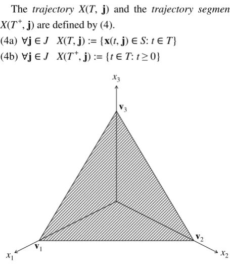
The (standard) 2-simplex (S), which is defined by
(1), is a triangle in ℝ3, as depicted by Figure 1. The
Cartesian coordinates of the simplex vertices v1, v2, and
v3 are stated by (2).
(1) S := {(x1, x2, x3) ∈ℝ3: x1 + x2 + x3 = 1 ∧∀i∈ {1, 2,
3} 0 ≤ xi≤ 1}
(2a) v1 := (1, 0, 0)
(2b) v2 := (0, 1, 0)
(2c) v3 := (0, 0, 1)
We define the vector functionx(t, j) as follows:
(3a) x(t, j) ≡ (x1(t, j), x2(t, j), x3(t, j)): T × J→ S
(3b) 0 ∈T⊆ℝ
(3c) J⊆S.
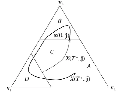
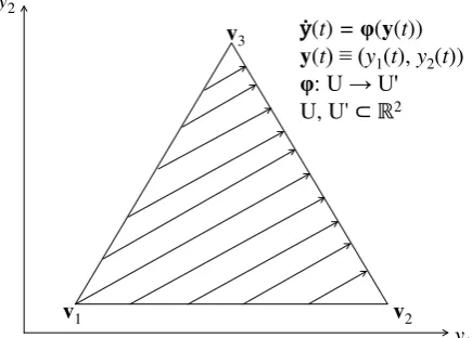
The trajectory X(T, j) and the trajectory segment X(T.+, j) are defined by (4).
(4a) ∀j∈J X(T,j) := {x(t, j) ∈S: t∈T}
(4b) ∀j∈J X(T +, j) := {t∈T: t ≥ 0}
x3
v3
v2 v1
[image:3.595.308.536.100.361.2]x2 x1
Figure 1. The standard simplex S in ℝ3.
In fact, (4a) defines a trajectory family indexed by
the set J, where each trajectory X(T,j) describes a path
on S that is traversed over the period T. X(T +, j) is the segment of this path that is traversed over t ≥ 0.
2.2 Set-Theoretical Trajectory Classification
(5) introduces a partitioning of S, which can be used
for describing the location of relevant trajectory points or segments (e.g., initial segment/state, empirically observed segment, or segment representing the future dynamics), as we will see later.
(5a) ∀i∈ {1, 2, 3} Svi := {(x1, x2, x3) ∈S: xi > 1/2}
(5b) Sv0 := S \ (Sv1∪Sv2∪Sv3)
(5a) and (1) imply that the partition Svi contains all
the points of S that are dominated by xi; i.e., if a point
(x1, x2, x3) is located in partition Svi, then ∀j∈ {1, 2, 3}\i
xi > xj. The geometrical interpretation of the partition-
ning (5) is depicted in Figure 2. As we can see, for i∈
{1, 2, 3}, the partition Svi contains all the points of S
that are closer to the vertex vi than to the other vertices
2 31 1 3
1 23 3 2
3 12 2 1
v w v v
v w v v
v w v v
⊥ ⊥ ⊥
Sv1 Sv2
Sv3
Sv0
v3
v2 v1
w31 w23
[image:4.595.69.273.93.264.2]w12
Figure 2. The partitioning of S.
The following (set-theoretical) definitions allow us to assess the prediction range of monotonous models, as we will see later. Let a(K) denote the area function
assigning the to a set K⊆S the (real number indicating
the) area of K. B(T, F) := ⋃j∈FX(T,j) is the image of the
family F of trajectories X(T, j), j ∈ F ⊆ J (cf. (4)).
Among all the path-connected and closed subsets of S
that cover B(T, F), let M(T, F) denote one of the sets
that cover the smallest area of S. a*(T, F) := a(M(T, F))
is the family image size of the family F.
2.3 Differential-Geometrical Trajectory Classification
While the previous discussion can be used for a set-theoretical characterization of trajectories, we focus now on a differential-geometrical characterization of trajectories referring to the angles of the tangential vectors and expressing the monotonicity characteristics and the curvature of a trajectory.
We say that the trajectory X(T,j) is continuous if for
the given j, x(t, j) is continuous in t on the time interval T (cf. (4a)). Moreover, a trajectory family is continuous
if all the trajectories belonging to this family are continuous.
Let (a) d(t, j) be the directional (or tangential) vector associated with the point x(t, j), (b) ℓ be a line
through the point x(t, j) that is parallel to the simplex
edge v1-v2, and (c) δ(t, j) := ∡(d(t, j), ℓ) ∈ [0°, 360°] be
the angle between the directional vector d(t, j) and the
line ℓ (cf. Figure 3).
X(T, j)
ℓ||
x(t, j)
d(t, j)
δ(t, j)
v2
v1
[image:4.595.321.522.131.293.2]v3
Figure 3. The vector angle δ(t, j).
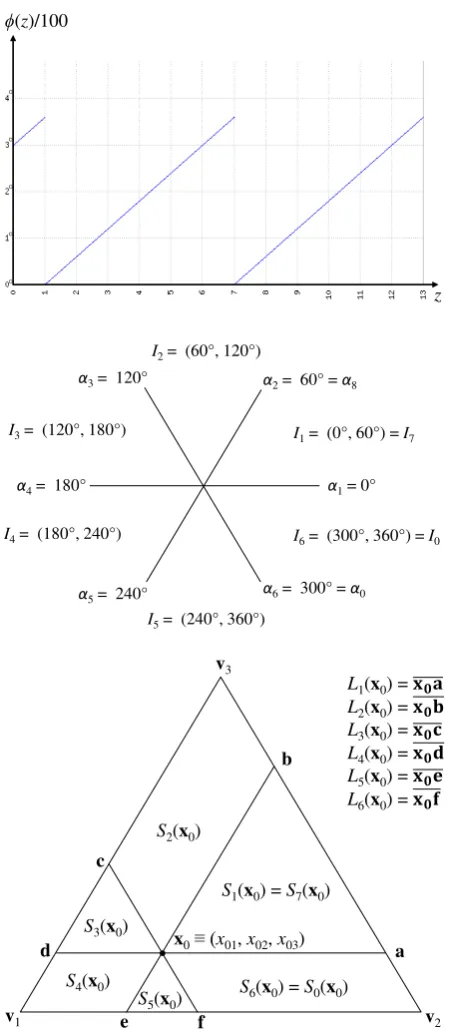
Moreover, we define the angles αi and the angle
intervals Ii by relying on the ‘saw tooth’ function ϕ: ℝ →ℝ as follows (cf. Figure 4):
(6a) ϕ(z) = [(z – 1)/6 – floor((z – 1)/6)]360°
(6b) ∀i∈ℕ Ii≡ (αi, αi+1) := (ϕ(i), ϕ(i + 1))
(6c) ∀i∈ℕ∀j∈ {n∈ℕ: i < n} [Ii~j] := ⋃ j
k = i [Ik] ∧
[Ii~j) := ⋃ j
k = i [Ik] \ αj+1 ∧ (Ii~j]:= ⋃ j
k = i [Ik] \ αi ∧ Ii~j := ⋃
j
k = i [Ik] \ αi\ αj+1
By using our definition of the vector angle δ(t, j) and
the vector angles and intervals (6), we can formulate the Properties 1-3 reflecting the relation between the tangential vector angles and the dynamics of x(t, j) in the case that ẋ(t, j) ≠ 0 (cf. Figures 1, 3, and 4).
Property 1. Ifẋ(t, j) ≠ 0, then (a) δ(t, j) ∈I3~5⟺ ẋ1(t, j) > 0, (b)δ(t, j) ∈I0~2⟺ẋ1(t, j) < 0, and (c) δ(t, j)
∈ {α3, α6} ⟺ẋ1(t, j) = 0.
Property 2. If ẋ(t, j) ≠ 0, then (a) δ(t, j) ∈I5~7⟺ ẋ2(t, j) > 0, (b) δ(t, j) ∈I2~4⟺ẋ2(t, j) < 0, and (c) δ(t, j)
∈ {α2, α5} ⟺ẋ2(t, j) = 0.
Property 3. If ẋ(t, j) ≠ 0, then (a) δ(t, j) ∈I1~3⟺ ẋ3(t, j) > 0, (b) δ(t, j) ∈I4~6⟺ẋ3(t, j) < 0, and (c) δ(t, j)
ϕ(z)/100
z °
° ° ° °
α1= 0°
α2= 60° = α8 α3= 120°
α4= 180°
α5= 240° α6= 300° = α0
I6= (300°, 360°) = I0
I1= (0°, 60°) = I7 I2= (60°, 120°)
I3= (120°, 180°)
I4= (180°, 240°)
I5= (240°, 360°)
.
S5(x0) S6(x0) = S0(x0)
S4(x0)
S3(x0)
S2(x0)
S1(x0) = S7(x0)
v1 v2
v3
x0≡ (x01, x02, x03)
f e
d c
b
L1(x0) =
L2(x0) =
L3(x0) =
L4(x0) =
L5(x0) =
L6(x0) =
[image:5.595.60.285.91.608.2]a
Figure 4. The function ϕ(z), the angle intervals Ii, the
line segments Li(x0), and the sets Si(x0).
We rely on the following definitions of monotoni- city. First, xi(t, j) is monotonous (in t) if (∀t∈Tẋi(t, j)
≥ 0) or (∀t ∈ T ẋi(t, j) ≤ 0). Second, xi(t, j) is strictly
monotonous (in t) if either (∀t ∈Tẋi(t, j) > 0) or (∀t∈
T ẋi(t, j) < 0) but not both. Third, the trajectory X(T,j)
(associated with the function x(t, j)) is (strictly) mono- tonous in one dimension if (a) there exists an i∈ {1, 2,
3} such that xi(t, j) is (strictly) monotonous and (b) for
all k ∈ {1, 2, 3}\ixk(t, j) is not (strictly) monotonous.
Fourth, the trajectory X(T,j) is (strictly) monotonous in two dimensions if (a) there exist an i∈ {1, 2, 3} and
a k ∈ {1, 2, 3}\i such that xi(t, j) and xk(t, j) are
(strictly) monotonous and (b) xl(t, j) is not (strictly)
monotonous with l ∈ {1, 2, 3}\{i, k}. Fifth, the
trajectory X(T,j) is (strictly) monotonous (in three di- mensions) if ∀i∈ {1, 2, 3} xi(t, j) is (strictly) monoto-
nous.
Instead of using the curvature definition that is
widespread in differential geometry (and which is difficult to apply in the proofs of our theorems), we use the following definition of curvature relying on vector angles: Let β(q, r, j) denote the angle between the two tangential vectors d(q, j) and d(r, j) associated
with the (monotonous) trajectory X(T,j) on S (cf. (4)),
where q, r ∈T. Among all the tangential vector pairs
(d(t, j), d(s, j)) associated with the (monotonous)
trajectory X(T,j), where t, s∈T, let d(t*, j) and d(s*, j) be among the ones that are characterized by the largest angle β, i.e., β(t*, s*, j) =: κ(T, j) is maximal tangential
vector angle range associated with the trajectory X(T,
j). The grater κ(T, j), the greater the curvature of the
trajectory X(T, j). Obviously, a linear trajectory has curvature of 0. We say that a strictly monotonous trajectory X(T, j) (or a trajectory segment) that
describes a clockwise (counterclockwise) movement on S has a positive (negative) signed curvature and
write κ(T, j) > 0 (κ(T, j) < 0). Let F be a family of
trajectories X(T,j), j∈F ⊆ J (cf. (4)). Then, κ*(T, F) :=
max(cl({κ(T,j): j∈F})) is the maximum curvature of the family F on the time interval T.
2.4 Topological Trajectory Classification
by homeomorphisms. Moreover, it is deciding for the applicability of the Poincaré-Bendixson theory (cf. Section 5) that the 2-simplex is homeomorphic to a bounded (and closed) subset of a plane.
Two trajectories X(T,j) and X(U, k) are non-inter-
secting if X(T, j) ∩ X(U, k) = ∅, where U ⊆ ℝ.
Otherwise they are intersecting. A trajectory X(T,j) is
self-intersecting if ∃(r, s, t) ∈T 3r < s < t∧ x(r, j) =
x(t, j) ≠ x(s, j). Otherwise, the trajectory is non-self-
intersecting. According to this definition, a closed trajectory is self-intersecting. A trajectory X(T, j) is
transversally self-intersecting if ∃(t, s) ∈T 2t≠ s∧x(t,
j) = x(s, j) ∧δ(t, j) ≠ δ(s, j). Otherwise, the trajectory is transversally non-self-intersecting. According to this definition, a closed trajectory corresponding to a Jordan curve is transversally non-self-intersecting.
3. Implications of Monotonicity
In contrast to monotonous and bounded trajectories in ℝ2, monotonous trajectories on the 2-simplex can
have (a) a wide range of different shapes and (b) omega limit sets consisting of more than only one (fixed) point. In this section, we discuss the geometrical aspects of the transitional and limit dynamics associated with continuous trajectories that are monotonous in one, two, or three dimensions. As we will, see these geometrical properties have interesting applications in economic dynamics modeling.
3.1 General Properties of Monotonous Trajectories on the 2-Simplex
In this section, we show that continuous trajectories that are monotonous in three dimensions (two dimensions) are characterized by relatively low curvatures, allow for relatively weak waves, and are placed in relatively small subsets of the 2-simplex in comparison to the ‘related’ trajectories that are monotonous in two dimensions (one dimension). Propositions 1-3 and Corollary 1 summarize these results formally. The readers who are less interested in this formal discussion can also go directly to the
discussion of Figure 4 (see the paragraphs below Proposition 3), which elaborates on the intuitive/gra- phical interpretation of these geometrical properties.
Given a point x0 ≡ (x01, x02, x03) ∈ S, (7) defines
different subsets of S. As we will see (in Proposition 3),
each of the subsets S1-S6 defined by (7) corresponds to
the closure of one of the vector angle intervals I1-I6
defined by (6) and each of the line segments L1-L6
defined by (7) corresponds to one of the angles α1-α6
defined by (6) (cf. Figure 4).
(7a) L1(x0) := {(x1, x2, x3) ∈S: x1≤x01∧x3 = x03}
(7b) S1(x0) := {(x1, x2, x3) ∈S: x2≥x02∧x3≥x03}
(7c) L2(x0) := {(x1, x2, x3) ∈S: x1≤x01∧x2 = x02}
(7d) S2(x0) := {(x1, x2, x3) ∈S: x1≤x01∧x2≤x02}
(7e) L3(x0) := {(x1, x2, x3) ∈S: x1 = x01∧x2≤x02}
(7f) S3(x0) := {(x1, x2, x3) ∈S: x1≥x01∧x3≥x03}
(7g) L4(x0) := {(x1, x2, x3) ∈S: x1≥x01∧x3 = x03}
(7h) S4(x0) := {(x1, x2, x3) ∈S: x2≤x02∧x3≤x03}
(7i) L5(x0) := {(x1, x2, x3) ∈S: x1≥x01∧x2 = x02}
(7j) S5(x0) := {(x1, x2, x3) ∈S: x1≥x01∧x2≥x02}
(7k) L6(x0) := {(x1, x2, x3) ∈S: x1 = x01∧x2≥x02}
(7l) S6(x0) := {(x1, x2, x3) ∈S: x1≤x01∧x3≤x03}
(7m) S0(x0) := S6(x0) S7(x0) := S1(x0)
(7n) ∀i∈ℕ∀j∈ {n∈ℕ: i < n} Si~j(x0) := ⋃jk = i Sk(x0)
Proposition 1. Assume that (a) the trajectory X(T,
j) defined by (4a) is continuous and monotonous in one
dimension on S, (b) x(0, j) = x0≡ (x01, x02, x03) ∈S, and
(c) ∀t ∈ Tẋ(t, j) ≠ 0. Then, X(T,j) and X(T +, j) (cf.
(4b)) satisfy one and only one of the Condition Sets P11-P19, which are defined as follows (cf. (6) and (7)):
a) for i ∈{1, 2, …, 6}, Condition Set P1i is: (∀t∈T
δ(t, j) ∈ [I(i–1)~(i+1)]) ∧ (∃t∈Tδ(t, j) ∈I(i–1)~(i+1)) ∧ (∃(r,
s) ∈T 2 δ(r, j) ∈ [Ii–1) ∧ δ(s, j) ∈ (Ii+1]) ∧ X(T +, j) ⊂
S(i–1)~(i+1)(x0);
b) for i∈ {7, 8, 9}, Condition Set P1i is: (∀t∈T
δ(t, j) ∈ {αi–6,αi–3}) ∧ (∃(p, q) ∈T
2δ(
p, j) ∈ {αi–6} ∧
δ(q, j) ∈ {αi–6}) ∧ X(T +, j) ⊆Li–6(x0) ∪Li–3(x0).
Proof. As defined in Section 2, X(T,j) is monotono-
3}, the function xi(t, j) is monotonous while for all
other i, xi(t, j) is non-monotonous. Thus, for proving
Proposition 1, we have to consider only three alternative scenarios of monotonicity in one dimensi- on: (A) x1(t, j) is monotonous, (B) x2(t, j) is
monotonous, and (C) x3(t, j) is monotonous. Moreover,
since a monotonous function can be monotonously increasing or monotonously decreasing (or both), we have three alternative sub-scenarios for each of the three scenarios (A)-(C): (a) monotonously increasing, (b) monotonously decreasing, and (c) both, monotono- usly increasing and monotonously decreasing (which means constant). Thus, overall, we have nine sub-sce- narios: (Aa)-(Ac), (Ba)-(Bc), and (Ca)-(Cc). According to Properties 1-3, each of the Condition Sets P11-P19, to
which Proposition 1 refers, represents one of the nine sub-scenarios (Aa)-(Cc). For example, Condition Sets P12, P15, and P17 represent the sub-scenarios (Ca),
(Cb), and (Cc), respectively.
Consider first the sub-scenario (Ca), i.e., assume that
x3(t, j) increases monotonously. Property 3 and (6b)
imply that (8) is valid in sub-scenario (Ca). (8) (∀t∈Tδ(t, j) ∈ [I1~3]) ∧ (∃t∈Tδ(t, j) ∈I1~3)
Moreover, according to the definition of ‘monoto- nicity in one dimension’, to which Proposition 1 refers, (9) is valid in sub-scenario (Ca).
(9) x1(t, j) and x2(t, j) are non-monotonous.
The interval [I1~3], to which (8) refers, can be
partitioned into three subintervals [I1), [I2], and (I3].
Properties 1 and 2 and (6b) imply (10).
(10a) ∀t∈Tδ(t, j) ∈ (I3] ⇒x1(t, j) is monotonous.
(10b) ∀t∈Tδ(t, j) ∈ [I1) ⇒x2(t, j) is monotonous.
(10c) ∀t ∈ T δ(t, j) ∈ [I2] ⇒x1(t, j) and x2(t, j) are
monotonous.
The statements (10) imply statement (11).
(11) x1(t, j) or x2(t, j) is monotonous if for all t ∈ T, δ(t,
j) is within one and only one of the subintervals
[I1), [I2],and (I3].
(9) and (11) imply that over the period T, the
tangential vectors δ(t, j) cannot stay within one and the
same subinterval, i.e., at least one subinterval switch
must occur over the period T. Given the three
subintervals [I1), [I2], and (I3], the set of all possible
subinterval switches is: (i) switch from [I1) to [I2], (ii)
switch from [I1) to (I3], (iii) switch from [I2] to [I1), (iv)
switch from [I2] to (I3], (v) switch from (I3] to [I1), and
(vi) switch from (I3] to [I2]. We analyze now these
interval switches. In case (i), i.e., if
(1.) initially, the tangential vector angles are within the interval [I1) and
(2.) at some later time point, the tangential vector angles switch to the interval [I2],
x1(t, j) is monotonous (cf. Property 1). This
contradicts (9). Analogously, it can be shown that cases (iii), (iv), and (vi) contradict (9), since: in case (iii),
x1(t, j) is monotonous; in case (iv), x2(t, j) is monotono-
us; in case (vi), x2(t, j) is monotonous. Only, in cases
(ii) and (v), both, x2(t, j) and x1(t, j), are non-monotono-
us, which is consistent with (9). In each of the cases (ii) and (v), (12) is true.
(12) ∃(r, s) ∈T 2δ(r, j) ∈ [I1) ∧δ(s, j) ∈ (I3]
The fact that x3(t, j) increases monotonously in
sub-scenario (Ca) implies that ∀t≥ 0 x3(t, j) ≥ x3(0, j),
where x3(0, j) = x03 according to the assumptions made
in Proposition 1. In other words, in sub-scenario (Ca),
X(T +, j) ⊂ {(x1, x2, x3) ∈S: x3≥x03} =: SCa(x0) (cf. Pro-
position 1). If X(T +, j) ⊂SCa(x0)⇒ X(T +, j) ⊂S1~3(x0),
then (13) is valid in sub-scenario (Ca). (13) X(T +, j) ⊂S1~3(x0)
We prove now that X(T +, j) ⊂SCa(x0)⇒ X(T +, j) ⊂
S1~3(x0). Given the point x0 ≡ (x01, x02, x03) ∈ S (cf.
Proposition 1), the definition of SCa(x0) (and (1))
implies that (14)-(16) are true if x(t, j) ∈SCa(x0).
(14) Either x3(t, j) > x03orx3(t, j) = x03 but not both.
(15) x2(t, j) < x02or x2(t, j) > x02(or x2(t, j) = x02 ).
(16) x1(t, j) < x01or x1(t, j) > x01(or x1(t, j) = x01).
The statement (16) can be divided into the two (disjunctive) cases (17a) and (17b).
(17a) Either x1(t, j) > x01or x1(t, j) = x01 but not both.
(17b) x1(t, j) < x01
If (14), (15), and (17a) are true and x(t, j) ∈S, then
x(t, j) ∈S3(x0) (cf. (7f)). We consider now the cases in
which (14), (15), and (17b) are true. These cases are: (18a) x1(t, j) < x01∧x3(t, j) > x03∧x2(t, j) > x02
(18b) x1(t, j) < x01∧x3(t, j) > x03∧x2(t, j) < x02
(18c) x1(t, j) < x01∧x3(t, j) > x03∧x2(t, j) = x02
(18d) x1(t, j) < x01∧x3(t, j) = x03∧x2(t, j) > x02
(18e) x1(t, j) < x01∧x3(t, j) = x03∧x2(t, j) < x02
(18f) x1(t, j) < x01∧x3(t, j) = x03∧x2(t, j) = x02
Obviously, the cases (18e) and (18f) violate (1). Thus, if (18e) or (18f) is true, then x(t, j) ∉S. If (18b) or
(18c) is true and x(t, j) ∈S, then x(t, j) ∈ {(x1, x2, x3) ∈
S: x1 < x01∧x2≤ x02 ∧x3 > x03} =: Sbc(x0). If x(t, j) ∈
S2(x0), then x3(t, j) ≥ x03, since, otherwise, (1) is
violated (cf. (7d)). In other words, S2(x0) = {(x1, x2, x3)
∈S: x1≤ x01∧x2≤ x02∧x3≥x03}. Obviously, Sbc(x0) ⊂
S2(x0). Thus, if (18b) or (18c) is true and x(t, j) ∈ S,
then x(t, j) ∈ S2(x0). Analogously, if (18a), (18c), or
(18d) is true and x(t, j) ∈S, then x(t, j) ∈ {(x1, x2, x3) ∈
S: x1 < x01∧ x2≥x02∧x3≥x03} =: Sacd(x0). Moreover, if
x(t, j) ∈S1(x0), then x1(t, j) ≤x01, since, otherwise, (1) is
violated (cf. (7b)). In other words, S1(x0) = {(x1, x2, x3)
∈S: x1≤x01∧ x2≥x02∧x3≥x03}. Obviously, Sacd(x0) ⊂
S1(x0). Thus, if (18a), (18c), or (18d) is true and x(t, j) ∈
S, then x(t, j) ∈S1(x0). Overall, we have shown that if
x(t, j) ∈SCa(x0) ⊆S, then the statements (14)-(17) are
valid, which imply several feasible cases. In each of these cases, x(t, j) is in one of the sets S1(x0), S2(x0), and
S3(x0), i.e., x(t, j) ∈SCa(x0) ⇒x(t, j) ∈S1(x0) ∪S2(x0) ∪
S3(x0). This implies that X(T +, j) ⊂SCa(x0)⇒ X(T +, j)
⊂S1(x0) ∪S2(x0) ∪S3(x0), since X(T +, j) is the union of
the points x(t, j) ∈S for which the statements (14)-(17)
(and (1)) hold (cf. Proposition 1). According to (7n),
S1~3(x0) = S1(x0) ∪S2(x0) ∪S3(x0). This completes the
proof that X(T +, j) ⊂SCa(x0)⇒ X(T +, j) ⊂S1~3(x0).
By now, we have shown that in the sub-scenario (Ca), the statements (8), (12), and (13) must be true. These three statements reduce to Condition Set P12. It
can be shown in the same way that
(1.) the sub-scenarios (Cb) and (Cc) correspond to Condition Sets P15 and P17, respectively, and
(2.) each of the sub-scenarios (Ba)-(Cc) corresponds to one and only one of the Condition Sets P11, P13, P14,
P16, P18, and P19.
This completes the proof that each of the alternative (sub-)scenarios of monotonicity in one dimension (i.e., each of the sub-scenarios (Aa)-(Cc)) corresponds to one and only one of the Condition Sets P11-P19. ∎
Proposition 2. Assume that (a) the trajectory X(T,j)
defined by (4a) is continuous and monotonous in two dimensions on S, (b) x(0, j) = x0≡ (x01, x02, x03) ∈S,
and (c) ∀t∈Tẋ(t, j) ≠ 0. Then, X(T,j) and X(T +, j) (cf.
(4b)) satisfy one and only one of the Condition Sets P21-P26, where for i∈ {1, 2, …, 6}, Condition Set P2i
is: (∀t∈Tδ(t, j) ∈ [Ii~(i+1)]) ∧ (∃(r, s) ∈T 2δ(r, j) ∈ [Ii) ∧δ(s, j) ∈ (I(i+1)]) ∧ X(T +, j) ⊂Si~(i+1)(x0) (cf. (6)/(7)).
Proof. According to the definition of monotonicity in two dimensions, two of the functions x1(t, j), x2(t, j),
and x3(t, j) must be monotonous, while the remaining
one must be non-monotonous. Thus, we have to consider only three cases: (A) x1(t, j) and x2(t, j) are
monotonous (while x3(t, j) is non-monotonous), (B)
x1(t, j) and x3(t, j) are monotonous (while x2(t, j) is
non-monotonous), and (C) x2(t, j) and x3(t, j) are
monotonous (while x1(t, j) is non-monotonous). For
each of these cases, we must distinguish between four subcases. For example, in case (A), we can distinguish between the following subcases: (a) x1(t, j) and x2(t, j)
are monotonously increasing, (b) x1(t, j) is monotono-
usly increasing, while x2(t, j) is monotonously
decreasing, (c) x1(t, j) and x2(t, j) are monotonously
decreasing, and (d) x1(t, j) is monotonously decreasing,
while x2(t, j) is monotonously increasing. Subcases (a)
and (c) are infeasible, since they violate (1): for example, if x1(t, j) and x2(t, j) are monotonously incre-
asing, then x3(t, j) must be monotonously decreasing
(instead of being non-monotonous), since x1(t, j) + x2(t,
j) + x3(t, j) must be equal to 1 for all t. Thus, we must
Properties 1 and 2 imply that in subcase (b) of case (A), the statement (19) is valid (cf. (6)).
(19) ∀t∈Tδ(t, j) ∈ [I3~4]
Moreover, since case (A) requires that x3(t, j) is
non-monotonous, Property 3 implies that (20) is valid in case (A).
(20) ∃(r, s) ∈T 2ẋ3(r, j) > 0 ∧ẋ3(s, j) < 0
According to (6), the interval [I3~4], to which (19)
refers, can be partitioned into the following partitions: [I3), α4, and (I4]. Property 3 and (6) imply (21).
(21a) ∀t∈Tδ(t, j) ∈ [I3) ∨δ(t, j) ∈ [I3) ∪α4⇒∀t∈T ẋ3(t, j)≥ 0
(21b) ∀t∈Tδ(t, j) ∈ (I4] ∨δ(t, j) ∈α4∪ (I4] ⇒∀t∈T ẋ3(t, j) ≤ 0
(21c) ∀t∈Tδ(t, j) ∈α4⇒∀t∈Tẋ3(t, j) = 0
The statements (21) imply that if (19) and (20) are true, the tangential vectors δ(t, j) cannot stay within one
and only one of the subintervals [I3), [I3) ∪α4, α4, α4∪
(I4], and (I4] for all t ∈T. That is, there must occur a
switch from subinterval [I3) to subinterval (I4] or from
subinterval (I4] to subinterval [I3) over the period T.
Thus, (22) is valid.
(22) ∃(r, s) ∈T 2δ(r, j) ∈ [I3) ∧δ(s, j) ∈ (I4]
Since in subcase (b) of case (A), x1(t, j) increases
monotonously and x2(t, j) decreases monotonously, the
assumptions made in Proposition 2 and (4b) imply that
X(T +, j) ⊂ {(x1, x2, x3) ∈ S: x1 ≥ x01 ∧ x2 ≤ x02} =:
SAb(x0). SAb(x0) can be partitioned as follows: SAb(x0) =
SAb1(x0) ∪SAb2(x0), where SAb1(x0) ∩SAb2(x0) = ∅ and
SAb1(x0) := {(x1, x2, x3) ∈S: x1≥x01∧ x2≤x02∧ x3≥x03}
and SAb2(x0) := {(x1, x2, x3) ∈S: x1≥x01∧ x2≤x02∧ x3 <
x03}. We can see immediately that SAb1(x0) ⊂S3(x0) (cf.
(7f)) and SAb2(x0) ⊂S4(x0) (cf. (7h)). Thus, SAb(x0) ⊂
S3(x0) ∪ S4(x0). This result, (7n), and the previously
shown fact that X(T +, j) ⊂SAb(x0) imply (23).
(23) X(T +, j) ⊂S3~4(x0)
Overall, we have shown that in the subcase (b) of case (A), Condition Set P23 must be true (cf. (19), (22),
and (23)). Analogously, it can be shown that in all the feasible subcases of cases (A)-(C), one and only one of
the statements P21, P22, P24, P25, and P26 is true, which
proves Proposition 2. ∎
Proposition 3. Assume that (a) the trajectory X(T,j)
defined by (4a) is continuous and monotonous (in three dimensions) on S, (b) x(0, j) = x0≡ (x01, x02, x03) ∈S,
and (c) ∀t∈Tẋ(t, j) ≠ 0. Then, X(T,j) and X(T +, j) (cf.
(4b)) satisfy one and only one of the Condition Sets P31-P312, where (cf. (6) and (7)):
a) for i∈ {1, 2, …, 6}, Condition Set P3i is: (∀t∈T
δ(t, j) ∈ [Ii]) ∧ (∃s∈Tδ(s, j) ∈Ii) ∧ X(T +, j) ⊂Si(x0);
b) for i∈ {7, 8, …, 12}, Condition Set P3i is: ∀t∈T
δ(t, j) ∈ {αi–6} ∧ X(T +, j) ⊆Li–6(x0).
Proof. According to our definition of monotonicity
(in three dimensions), x1(t, j), x2(t, j), and x3(t, j) must
be monotonous if X(T, j) is monotonous (in three
dimensions) on S. Since a monotonous function can be
(a) monotonously increasing, (b) monotonously decreasing, or (c) both (monotonously increasing and monotonously decreasing and, thus, constant), we have per function xi(t, j) three cases ((a)-(c)). Moreover, we
have three functions x1(t, j), x2(t, j), and x3(t, j). Thus,
overall, there are 33 possible combinations. This set of 27 combinations contains the combination (A) ∀i ẋi(t,
j) ≤ 0, the combination (B) ∀iẋi(t, j) ≥ 0, three times the
combination (C) ẋi(t, j) ≥ 0 ∧ẋk(t, j) ≥ 0 ∧ẋl(t, j) = 0 ∧i
≠ k ≠ l, three times the combination (D) ẋi(t, j) ≤ 0 ∧
ẋk(t, j) ≤ 0 ∧ ẋl(t, j) = 0 ∧ i ≠ k ≠ l, six times the
combination (E) ẋi(t, j) = ẋk(t, j) = 0 ∧ẋl(t, j) ≠ 0 ∧i≠ k
≠ l, and the combination (F) ∀i ẋi(t, j) = 0. The
combinations (A)-(E) are infeasible, since they violate (1) unless they reduce to combination (F). The combination (F) represents a fixed point (ẋ(t, j) = 0)
and is excluded by the assumptions made in Propositi- on 3. In the rest of the proof, we have to consider the remaining 12 combinations.1 Each of these 12 combi-
1 These feasible combinations are: (1.) ẋ
nations is covered by one of the Conditions Sets P31-
P312. We leave it to the reader to prove the validity of
Proposition 3 in all these 12 cases; we prove the validity in only two representative cases. Consider the case ∀t∈Tẋ1(t, j) ≤ 0 ∧ẋ2(t, j) ≤ 0 ∧ẋ3(t, j) ≥ 0, where
∃(r, s, p) ∈T 3ẋ1(r, j) <0 ∧ẋ2(s, j) < 0 ∧ẋ3(p, j) > 0.
Then,
(a) Properties 1-3 imply almost directly that the tangential vector angles δ(t, j) satisfy the Condition Set
P32, and
(b) the assumptions made in Proposition 3 and (4b) imply that X(T +, j) ⊂ {(x1, x2, x3) ∈S: x1≤x01∧ x2≤x02
∧ x3≥x03} =: Sz(x0), and, thus, (7d) implies that Sz(x0)
⊂ S2(x0); thus, X(T +, j) ⊂ S2(x0) as stated by the
Condition Set P32.
Alternatively, consider the case ∀t∈Tẋ1(t, j) ≤ 0 ∧ ẋ2(t, j) ≥ 0 ∧ẋ3(t, j) = 0, where ∃r∈T ẋ1(r, j) < 0 ∧ ẋ2(r, j) > 0.2 Properties 1-3 imply almost directly that
in this case, the tangential vector angles δ(t, j) satisfy
the Condition Set P37. Moreover, the assumptions
made in Proposition 3, (4b), and (7a) imply that X(T +,
j) ⊆ {(x1, x2, x3) ∈S: x1≤x01∧ x2≥x02∧ x3 = x03} ⊆
L1(x0). Thus, X(T +, j) ⊆L1(x0) as stated by Condition
Set P37. ∎
We discuss now the geometrical interpretation of Properties 1-3 as depicted by Figure 4. To construct Figure 4, we choose an arbitrary point (x0) in the
interior of S. Then, we draw three line segments going
through x0 and each being parallel to one of the simplex
edges v1-v2, v2-v3, and v3-v1. The intersections of the
line segments with the simplex edges are denoted by the points a-f. We can see that the line segments that connect x0 with one of the points a-f are the line
segments L1(x0)-L6(x0), which are defined by (7) and
which localize the six (closed) subsets S1(x0)-S6(x0)
defined by (7). The angles between the line segments
0, where ∃t ∈ T ẋi(t) < 0 if it is stated that ẋi ≤ 0, and, analogously, ∃t∈Tẋi(t) >0 if it is stated that ẋi ≥0.
2 Note that the cases ẋ
1(r, j) < 0 ∧ẋ2(r, j) = ẋ3(r, j) = 0 and ẋ2(r,
j) > 0 ∧ẋ1(r, j) = ẋ3(r, j) = 0 are infeasible (see the discussion of combinations (A)-(E)).
L1(x0)-L6(x0) and the simplex edge v1-v2 (according to
the definition of tangential vector angles and intervals (6)) are depicted in the middle panel of Figure 4. (7n) and Figure 4 imply almost directly that
(1.) each of the six sets Si~(i+1)(x0), to which
Proposition 2 refers, is simply the union of two neighboring sets Sj(x0) and Sk(x0),
(2.) each of the six sets S(i–1)~(i+1)(x0), to which
Proposition 1 refers, is simply the union of three neighboring sets Sj(x0), Sk(x0), and Sm(x0).
In particular, Propositions 1-3 can be interpreted easily by using Figure 4:
1.) Proposition 3 implies three geometrical proper- ties of a trajectory segment X(T +, j) that is monotonous
in three dimensions. First, X(T +, j) is located in one of
the line segments L1(x0)-L6(x0) or in one of the sets
S1(x0)-S6(x0). Second, if X(T +, j) is in Li(x0), then for all
t≥ 0, the tangential vector angles δ(t, j) associated with
X(T +, j) are equal to the angle that is associated to the
line segment Li(x0) in Figure 4 +/–180°. For example, if
X(T +, j) is in L3(x0), then δ(t, j) ∈ {120°, 300°} for t≥ 0.
Third, if X(T +, j) is located in one of the sets Si(x0), then
for t≥ 0, the tangential vector angles δ(t, j) associated with X(T +, j) are within the angle range indicated by
the angles associated to the line segments Li(x0) and
Li+1(x0) that bound the set Si(x0) in Figure 4. For
example, if the trajectory segment X(T +, j) that is mo-
notonous in three dimensions is in S3(x0), then δ(t, j) is
within the angle range [120°, 180°] for t ≥ 0 (cf.
Proposition 3 and Condition Set P33).
2.) The geometrical interpretation of Proposition 2 is analogous. In particular, the trajectory segment X(T +, j)
that is monotonous in two dimensions is located in two neighboring sets Sj(x0) and Sk(x0), and for all t≥ 0, the
tangential vector angles δ(t, j) of X(T +, j) are within the
angle range indicated by the angles associated to the two line segments Lj(x0) and Lk+1(x0) that bound the
union of the sets Sj(x0) and Sk(x0) in Figure 4. For
example, if the trajectory segment X(T +, j) that is mo-
S4(x0), then δ(t, j) is within the angle range [120°, 240°]
for t≥ 0 (cf. Proposition 2 and Condition Set P23).
3.) Analogously, Proposition 1 implies that the trajectory segment X(T +, j) that is monotonous in one
dimension is located in three neighboring sets Sj(x0),
Sk(x0), and Sm(x0). Moreover, for all t≥ 0, the tangential
vector angles δ(t, j) associated with this trajectory
segment are within the angle range indicated by the angles associated to the two line segments Lj(x0) and
Lm+1(x0) that bound the union of the sets Sj(x0), Sk(x0),
and Sm(x0) in Figure 4. For example, if the trajectory
segment X(T +, j) that is monotonous in one dimensions
is in S3~5(x0) = S3(x0) ∪S4(x0) ∪S4(x0), then δ(t, j) is
within the angle range [120°, 300°] for t ≥ 0 (cf.
Proposition 1 and Condition Set P14).
This graphical interpretation highlights important implications of Propositions 1-3: First, a trajectory that is monotonous (in three dimensions) is captured in a smaller subset of S than a related trajectory that is
monotonous in two dimensions. Second, a trajectory that is monotonous in two dimensions is captured in a smaller subset of S than a related trajectory that is
monotonous in one dimension. Moreover, the
maximum curvature κ*
of trajectories that are monotonous in three dimensions (two dimensions) is
greater than the maximum curvature of related
trajectories that are monotonous in two dimensions (one dimension).
This intuitive discussion does not explicitly define the meaning of the term ‘related’. Thus, we define the meaning of this term and then formulate Corollary 1 (which is implied by Propositions 1-3) on the basis of this definition such that the discussion becomes more precise. Let F(x0) ⊆ J be a family of continuous trajec-
tory segments X(T +, j) ⊂S,j∈ F(x0), satisfying ∀j∈
F(x0) x(0,j) = x0∈S and ∀t ∈ T +∀j∈ F(x0) ẋ(t, j) ≠ 0
(cf. (4)). Moreover, let P11(x0), P12(x0), …, P16(x0),
P21(x0), P22(x0), …, P26(x0), P31(x0), P32(x0), …, and
P36(x0) denote the subfamilies of F(x0) satisfying the
Conditions Sets P11, P12, …, P16, P21, P22, …, P26,
P31, P32, …, and P36, respectively. That is, j∈Pcd(x0)
⊂ F(x0) implies that X(T +, j) satisfies the Condition Set
Pcd, where c∈ {1, 2, 3} and d∈ {1, 2, …, 6}. For (h, k) ∈ {1, 2, …, 6}2, we say that the families P1h(x0) and
P2k(x0) are related if ∃i ∈ {1, 2, 3} ∀j ∈ P1h(x0) ∪
P2k(x0) (∀t ∈ T +ẋi(t, j) ≥ 0) ∨ (∀t ∈ T +ẋi(t, j) ≤ 0)∧ (∃tj
∈ T + ẋi(tj, j) ≠ 0). That is, a family defined by
Proposition 1 is related to a family defined by Proposi-
tion 2 if there exists an i for which the monotonicity
characteristics of xi(t, j) are identical in both families.
For example, the families P12(x0) and P21(x0) are
characterized by a monotonously increasing x3(t, j),
i.e., ∀j∈P12(x0) ∪P21(x0) (∀t ∈ T +ẋ3(t, j) ≥ 0) ∧ (∃tj∈
T +ẋ3(tj, j) > 0); thus, P12(x0) and P21(x0) are related.
We define the relations between the families defined by Propositions 2 and 3 analogously: For (p, q)∈{1, 2, …,
6}2, we say that the families P2p(x0) and P3q(x0) are
related if ∃(v, w) ∈ {1, 2, 3}2 ∀j ∈P2p(x0) ∪P3q(x0)
(∀t ∈ T +ẋv(t, j) ≥ 0) ∨ (∀t ∈ T +ẋv(t, j) ≤ 0)∧ (∀t ∈ T +
ẋw(t, j) ≥ 0) ∨ (∀t ∈ T +ẋw(t, j) ≤ 0)∧ (∃tj∈ T +ẋv(tj, j) ≠
0) ∧ (∃sj∈ T +ẋi(sj, j) ≠ 0) ∧ v≠ w. That is, a family
defined by Proposition 2 is related to a family defined
by Proposition 3 if (a) there exists a v for which the
monotonicity characteristics of xv(t, j) are identical in
both families and (b) there exists a w≠ v for which the
monotonicity characteristics of xw(t, j) are identical in
both families. For example, as implied by (6), Properties 1 and 3, and Propositions 2 and 3, the families P21(x0) and P31(x0) are characterized by (a) a
monotonously decreasing x1(t, j), i.e., ∀j∈ P21(x0) ∪
P31(x0) (∀t ∈ T +ẋ1(t, j) ≤ 0) ∧ (∃tj∈ T +ẋ1(tj, j) < 0),
and (b) a monotonously increasing x3(t, j), i.e., ∀j ∈
P21(x0) ∪P31(x0) (∀t ∈ T +ẋ3(t, j) ≥ 0) ∧ (∃sj∈ T +ẋ3(sj,
j) > 0). Thus, P21(x0) and P31(x0) are related.
Corollary 1. a) Consider the trajectory family
P1h(x0), where h∈ {1, 2, …, 6} and x0≡ (x01, x02, x03) ∈
int(S). There exist two trajectory families P2k(x0) and
P2m(x0), (k, m)∈{1, 2, …, 6}2, k ≠ m, that are related to
P1h(x0) and satisfy the following condition: ∀n ∈{k,
m} a*(T +, P1h(x0)) > a*(T +, P2n(x0)) ∧ κ*(T +,
b) Consider the trajectory family P2p(x0), where p∈
{1, 2, …, 6} and x0≡ (x01, x02, x03) ∈ int(S). There exist
two trajectory families P3q(x0) and P3r(x0), (q, r)∈{1,
2, …, 6}2, q ≠ r, that are related to P2p(x0) and satisfy
the following condition: ∀u ∈{q, r} a*(T +, P2p(x0)) >
a*(T +, P3u(x0))∧κ*(T +, P2p(x0))>κ*(T +, P3u(x0)).
Proof. We only sketch here the proof. Starting with Corollary 1a, assume that h = 2, i.e., consider the
family P12(x0). According to our definition of
relatedness, P12(x0) is related to P21(x0) and P22(x0),
since (6), Property 3, and Propositions 1 and 2 imply that P12(x0), P21(x0), and P22(x0) are characterized by a
monotonously increasing x3(t, j).
According to Proposition 1, (7b), (7d), (7f), (7n), and the definitions of a and M given in Section 2.2, the
following statements are true:
(24) M(T +, P12(x0)) ⊆ S1~3(x0) = S1(x0) ∪ S2(x0) ∪
S3(x0) = {(x1, x2, x3) ∈S: x3≥x03}
(25) M(T +, P21(x0)) ⊆ S1~2(x0) = S1(x0) ∪ S2(x0) ⊂
S1~3(x0)
(26) M(T +, P22(x0)) ⊆ S2~3(x0) = S2(x0) ∪ S3(x0) ⊂
S1~3(x0)
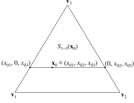
As implied by (24), all the trajectories belonging to the family P12(x0) are located in S1~3(x0), where the
latter is a triangle obtained by constructing a line on S
going through x0 and being parallel to the simplex edge
v1-v2 (cf. Property 3a, (6), and Figures 3 and 5).
According to Proposition 1 and (6), all the trajectories belonging to the family P12(x0) satisfy the following
vector angle condition:
(27) ∀j∈P12(x0) (∀t∈T +δ(t, j) ∈ [0°, 180°]) ∧ (∃(r,
s) ∈T + × T +δ(r, j) ∈ [0°, 60°) ∧δ(s, j) ∈ (120°, 180°])
If we allow for non-smooth trajectories and, in
particular, trajectories that are unions of line segments, it is easy to show geometrically by referring to Figure 5 that such trajectories can be constructed to any point on
S1~3(x0) while satisfying the condition (27).3 Thus,
3 Exactly speaking, (a) each of the line segments constituting
such a trajectory is characterized by an angle to the v1-v2-edge of S in the range of [0°, 180°], (b) each trajectory contains a
M(T +, P12(x0)) = S1~3(x0) and, thus, a*(T +, P12(x0)) =
a(S1~3(x0)) (cf. Section 2.2). Moreover, (25) and (26)
imply that a*(T +, P21(x0)) ≤ a(S1~2(x0)) < a(S1~3(x0))
and a*(T +, P22(x0))) ≤ a(S2~3(x0)) < a(S1~3(x0)). Thus,
(28) is true.
(28) a*(T +, P12(x0)) > a*(T +, P21(x0)) ∧a*(T +, P12(x0))
> a*(T +, P22(x0)).
If we require that the trajectories belonging to the family P12(x0) are smooth (i.e., ∀j ∈P12(x0) ∀t∈T +
x(t, j) is differentiable with respect to t), then it is not
possible to construct a trajectory that obeys (27) and goes through the points/vertices (x01, 0, x03) ∈S1~3(x0)
and (0, x02, x03) ∈S1~3(x0), which can be easily proven
by referring to Figures 4 and 5. That is, the smooth trajectories belonging to the family P12(x0) cannot
cover two infinitesimally small areas of S1~3(x0).
However, even in this case, it is still ensured that a*(T +, P12(x0)) > a*(T +, P21(x0)), since
(a) S1~3(x0) = S1~2(x0) ∪S3(x0) (cf. (24) and (25)),
(b) S3(x0) (cf. (24)) is not infinitesimally small (in
generic cases), and
(c) a*(T +, P21(x0)) ≤ a(S1~2(x0)).
The definition of κ*
(cf. Section 2.3) and (27) imply that κ*
(T +, P12(x0)) = 180°. Analogously, Proposition
2, definition of κ*, and (6) imply that κ*(
T +, P21(x0)) =
120°. Thus, κ*
(T +, P12(x0)) > κ*(T +, P21(x0)).
Overall, by now we have (heuristically) proven Corollary 1a for h = 2. The proof is analogous for h∈
{1, 3, 4, 5, 6}. The proof of Corollary 1b is very similar to the proof of Corollary 1a. Thus, we omit it here. ∎
Overall, among related trajectories and trajectory families the following is true: the higher the dimension of monotonicity, the smaller is (a) the family image (and, thus, the set of predicted states) and (b) the maximal curvature and (and, thus, the potential strength of waves).
If two families are unrelated, then a higher degree of monotonicity does not necessarily imply a smaller family image and a smaller maximum curvature.
.
S1~3(x0)
v1 v2
v3
x0≡ (x01, x02, x03)
.
.
[image:13.595.61.280.146.315.2](x01, 0, x03) (0, x02, x03)
Figure 5. The set S1~3(x0).
We can see that Corollary 1 does not categorize all the Condition Sets postulated by Propositions 1 and 3 and, in particular, not the Condition Sets P17-P9 and
P37-P312. These Condition Sets imply that one of the
xi(t, j) is constant for all t∈T
+ and, thus, the trajectory
segments X(T +, j) are located on line segments. Obvi- ously, the constancy requirement is much stronger than a monotonicity requirement, thus, in the cases repre- sentted by the Condition Sets P17-P9 and P37-P312, the
size of the family image M(.) is relatively small and the
curvature is zero.
3.2 Implications for Prediction of Transitional Dynamics
If we regard t = 0 as now and t > 0 as the future (and,
thus, T + as the predicted trajectory segment), Corollary
1 implies that the trajectories that are monotonous in one dimension (two dimensions) are harder to predict than the trajectories that are monotonous in two dimensions (three dimensions), ceteris paribus, since (a) the set of all possible future states is relatively great and (b) relatively stronger curvatures/waves may arise in the former case (in comparison to the latter case).
However, besides the monotonicity characteristics, the location of the initial state x0 is decisive for the
predictability of the future dynamics. In particular, the family image M and its size a* depend on x0 (cf.
Corollary 1 and its proof). In general, monotonicity
implies that the system moves from x0 along the
trajectory segment T + towards a vertex or an edge of
the 2-simplex. Thus, if the initial state x0 is relatively
close to this vertex/edge, T + is captured in a relatively
small set, i.e., the set of potential future states of the system is relatively small. This is almost a direct implication of the boundedness of the 2-simplex.
As implied by Propositions 1-3, (6), and Section 2.3 (cf. Proof of Corollary 1), the maximum curvature κ*
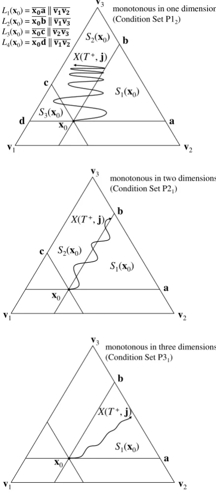
of trajectories that are monotonous in three dimensions, two dimensions, and one dimension is 60°, 120°, and 180°, respectively. Thus, the cyclical behavior corres- ponding to a (transversally) self-intersecting or closed trajectory (Jordan curve) is prohibited in all cases of monotonicity, since this type of cyclical behavior requires a curvature greater than 180°. Yet, monotonous trajectories allow for cyclical behavior corresponding to waves on the simplex (see Figure 6).
The angle range of 180° associated with
monotonicity in one dimension allows for waves of
high amplitude and short wavelength on the 2-simplex. In contrast, monotonicity in three dimensions allows
only for relatively low-amplitude/long-wavelength waves (cf. Figure 6).
Obviously, all three types of monotonicity allow for curved trajectories on the 2-simplex. However, only monotonicity in three dimensions allows for unidirectional linear trajectories, while monotonicity in one dimension allows for linear trajectories yet requires at least one direction change.
3.3 Limit Dynamics
Jordan curve are excluded, since such cycles require that x1(t), x2(t), and x3(t) are non-monotonous in the
limit. Second, the system may converge to a fixed point or reach the fixed point in finite time (and stay there). The proof of these facts is obvious.
.
S3(x0)
S2(x0)
S1(x0)
v1 v2
v3
x0
d c
b
L1(x0) = ||
L2(x0) = || L3(x0) = ||
L4(x0) = ||
a
X(T+, j)
monotonous in one dimension (Condition Set P12)
.
S2(x0)
S1(x0)
v1 v2
v3
x0 c
b
a
X(T+, j)
monotonous in two dimensions (Condition Set P21)
.
S1(x0)v1 v2
v3
x0
b
monotonous in three dimensions (Condition Set P31)
a
[image:14.595.60.280.173.675.2]X(T+, j)
Figure 6. Examples of monotonous waves.
In the case of monotonicity in three dimensions, only the fixed point outcome is possible, as implied by the monotone convergence theorem: since each of the functions x1(t), x2(t), and x3(t) is monotonous and
restricted by an upper/lower limit of 0 and 1, each of the x1(t), x2(t), and x3(t) converges to its fixed point (x1*,
x2*, and x3*, respectively) or reaches it in finite time
(and stays there). Thus, x(t) converges to a fixed point
x*≡ (x1*, x2*, x3*) ∈S or reaches it in finite time.
Additionally, in the case of monotonicity in one dimension, the system may converge to a line segment if the trajectory is a wave. In this case, the wavelength decreases and the vector-angle range converges to the range of 180° as the system converges to the line segment (see the first part of Figure 6).
Note that in the case of monotonicity in two dimensions, the convergence to a line segment is not possible, as explained in the following. If the trajectory converges to a line segment, the tangential vector angle range must increase to a range of 180° which is prohibited by the definition of monotonicity in two dimensions, which allows only for a vector angle range of 120°. The former fact follows from the definition of the omega limit set, where for each of the points on the line segment (constituting the omega limit set), a sequence of points on the wave must be found that converges to it.