Word Sense Clustering and Clusterability

Diana McCarthy

Marianna Apidianaki

LIMSI, CNRS, Universit´e Paris-Saclay

Katrin Erk

University of Texas at Austin

Word sense disambiguation and the related field of automated word sense induction tradi-tionally assume that the occurrences of a lemma can be partitioned into senses. But this seems to be a much easier task for some lemmas than others. Our work builds on recent work that proposes describing word meaning in a graded fashion rather than through a strict partition into senses; in this article we argue that not all lemmas may need the more complex graded analysis, depending on their partitionability. Although there is plenty of evidence from previous studies and from the linguistics literature that there is a spectrum of partitionability of word meanings, this is the first attempt to measure the phenomenon and to couple the machine learning literature on clusterability with word usage data used in computational linguistics.

We propose to operationalize partitionability as clusterability, a measure of how easy the occurrences of a lemma are to cluster. We test two ways of measuring clusterability: (1) existing measures from the machine learning literature that aim to measure the goodness of optimal k-means clusterings, and (2) the idea that if a lemma is more clusterable, two clusterings based on two different “views” of the same data points will be more congruent. The two views that we use are two different sets of manually constructed lexical substitutes for the target lemma, on the one hand monolingual paraphrases, and on the other hand translations. We apply automatic clustering to the manual annotations. We use manual annotations because we want the representations of the instances that we cluster to be as informative and “clean” as possible. We show that when we control for polysemy, our measures of clusterability tend to correlate with partitionability, in particular some of the type-(1) clusterability measures, and that these measures outperform a baseline that relies on the amount of overlap in a soft clustering.

∗Department of Theoretical and Applied Linguistics, University of Cambridge, UK. E-mail:diana@dianamccarthy.co.uk.

∗∗LIMSI, CNRS, Universit´e Paris-Saclay, France. E-mail:marianna.apidianaki@limsi.fr.

†Department of Linguistics, University of Texas at Austin, USA. E-mail:katrin.erk@mail.utexas.edu. Submission received: 13 June 2014; revised version received: 3 August 2015; accepted for publication: 25 January 2016.

1. Introduction

In computational linguistics, the field of word sense disambiguation (WSD)—where a computer selects the appropriate sense from an inventory for a word in a given context—has received considerable attention.1Initially, most work focused on manually constructed inventories such as WordNet (Fellbaum 1998) but there has subsequently been a great deal of work on the related field of word sense induction (WSI) (Pedersen 2006; Manandhar et al. 2010; Jurgens and Klapaftis 2013) prior to disambiguation. This article concerns the phenomenon of word meaning and current practice in the fields of WSDandWSI.

Computational approaches to determining word meaning in context have tradi-tionally relied on a fixed sense inventory produced by humans or by aWSIsystem that groups token instances into hard clusters. Either sense inventory can then be applied to tag sentences on the premise that there will be one best-fitting sense for each token instance. However, word meanings do not always take the form of discrete senses but vary on a continuum between clear-cut ambiguity and vagueness (Tuggy 1993). For example, the nouncraneis a clear-cut case of ambiguity between lifting device and bird, whereas the exact meaning of the nounthingcan only be retrieved via the context of use rather than via a representation in the mental lexicon of speakers. Cases of polysemy such as the verbpaint, which can mean painting a picture, decorating a room, or painting a mural on a house, lie somewhere between these two poles. Tuggy highlights the fact that boundaries between these different categories are blurred. Although specific context clearly plays a role (Copestake and Briscoe 1995; Passonneau et al. 2010) some lemmas are inherently much harder to partition than others (Kilgarriff 1998; Cruse 2000). There are recent attempts to address some of these issues by using alternative characterizations of word meaning that do not involve creating a partition of usages into senses (McCarthy and Navigli 2009; Erk, McCarthy, and Gaylord 2013), and by asking WSIsystems to produce soft or graded clusterings (Jurgens and Klapaftis 2013) where tokens can belong to a mixture of the clusters. However, these approaches do not overtly consider the location of a lemma on the continuum, but doing so should help in determining an appropriate representation. Whereas the broad senses of the nouncrane could easily be represented by a hard clustering, this would not make any sense for the nounthing; meanwhile, the verbpaintmight benefit from a more graded representation. In this article, we propose the notion ofpartitionabilityof a lemma, that is, the ease with which usages can be grouped into senses. We exploit data from annotation studies to explore the partitionability of different lemmas and see where on the ambiguity– vagueness cline a lemma is. This should be useful in helping to determine the appro-priate computational representation for a word’s meanings—for example, whether a hard clustering will suffice, whether a soft clustering would be more appropriate, or whether a clustering representation does not make sense. To our knowledge, there has been no study on detecting partitionability of word senses.

We operationalize partitionability asclusterability, a measure of how much struc-ture there is in the data and therefore how easy it is to cluster (Ackerman and Ben-David 2009a), and test to what extent clusterability can predict partitionability. For deriving a gold estimate of partitionability, we turn to the Usage Similarity (hereafterUsim) data set (Erk, McCarthy, and Gaylord 2009), for which annotators have rated the similarity of

pairs of instances of a word using a graded scale (an example is given in Section 2.2). We use inter-annotator agreement (IAA) on this data set as an indication of partitionability. Passonneau et al. (2010) demonstrated that IAA is correlated with sense confusability. Because this data set consists of similarity judgments on a scale, rather than annotation with traditional word senses, it gives rise to a second indication of partitionability: We can use the degree to which annotators have used intermediate points on a scale, which indicate that two instances are neither identical in meaning nor completely different, but somewhat related.

We want to know to what extent measures of clusterability of instances can predict the partitionability of a lemma. As our focus in this article is to test the predictive power of clusterability measures in the best possible case, we want the representations of the instances that we cluster to be as informative and “clean” as possible. For this reason, we represent instances through manually annotated translations (Mihalcea, Sinha, and McCarthy 2010) and paraphrases (McCarthy and Navigli 2007). Both translations (Resnik and Yarowsky 2000; Carpuat and Wu 2007; Apidianaki 2008) and monolingual paraphrases (Yuret 2007; Biemann and Nygaard 2010; Apidianaki, Verzeni, and McCarthy 2014) have previously been used as a way of inducing word senses, so they should be well suited for the task. Since the suggestion by Resnik and Yarowsky (1997) to limit WSD to senses lexicalized in other languages, numerous works have exploited translations for semantic analysis. Dyvik (1998) discovers word senses and their relationships through translations in a parallel corpus and Ide, Erjavec, and Tufis¸ (2002) group the occurrences of words into senses by using translation vectors built from a multilingual corpus. More recent works focus on discovering the relationships between the translations and grouping them into clusters either automatically (Bannard and Callison-Burch 2005; Apidianaki 2009; Bansal, DeNero, and Lin 2012) or manually (Lefever and Hoste 2010). McCarthy (2011) shows that overlap of translations compared to overlap of paraphrases on sentence pairs for a given lemma are correlated with inter-annotator agreement of graded lemma usage similarity judgments (Erk, McCarthy, and Gaylord 2009) but does not attempt to cluster the translation or paraphrase data or examine the findings in terms of clusterability. In this initial study of the clusteribility phenomenon, we represent instances through translation and paraphrase annotations; in the future, we will move to automatically generated instance representations.

should be computationally easier to cluster (Ackerman and Ben-David 2009b) because the structure in the data is more obvious, so any reasonable algorithm should be able to partition the data to reflect that structure. We contrast the performance of the three intra-clust measures and the inter-intra-clust measure with a simplistic baseline that relies on the amount of overlapping items in a soft clustering of the instance data, since such a baseline would be immediately available if one applied soft clustering to all lemmas.

We show that when controlling for polysemy, our indicators of higher clusterability tend to correlate with our two gold standard partitionability estimates. In particular, clusterability tends to correlate positively with higher inter-annotator agreement and negatively with a greater proportion of mid-range judgments on a graded scale of instance similarity. Although all our measures show some positive results, it is the intra-clust measures (particularly two of these) that are most promising.

2. Characterizing Word Meaning

2.1 The Difficulty of Characterizing Word Meaning

There has been an enormous amount of work in the fields ofWSDandWSIrelying on a fixed inventory of senses and on the assumption of a single best sense for a given instance (for example, see the large body of work described in Navigli [2009]) though doubts have been expressed about this methodology when looking at the linguistic data (Kilgarriff 1998; Hanks 2000; Kilgarriff 2006). One major issue arises from the fact that there is a spectrum of word meaning phenomena (Tuggy 1993) from clear-cut cases of ambiguity where meanings are distinct and separable, to cases where meanings are intertwined (highly interrelated) (Cruse 2000; Kilgarriff 1998), to cases of vagueness at the other extreme where meanings are underspecified. For example, at the ambiguous end of the spectrum are words likebank(noun) with the distinct senses of financial in-stitution and side of a river. In such cases, it is relatively straightforward to differentiate corpus examples and come up with clear definitions for a dictionary or other lexical resource.2These clearly ambiguous words are commonplace in articles promotingWSD because the ambiguity is evident and the need to resolve it is compelling. On the other end of the spectrum are cases where meaning is unspecified (vague); for example, Tuggy gives the example thataunt can be father’s sister or mother’s sister. There may be no contextual evidence to determine the intended reading and this does not trouble hearers and should not trouble computers (the exact meaning can be left unspecified). Cases of polysemy are somewhere in between. Examples from Tuggy include the noun set (a chess set, a set in tennis, a set of dishes, and a set in logic) and the verbbreak(a stick, a law, a horse, water, ranks, a code, and a record), each having many connections between the related senses. Although it is assumed in many cases that one meaning has spawned the other by a metaphorical process (Lakoff 1987)—for example, the mouth of a river from the mouth of a person—the process is not always transparent and neither is the point at which the spawned meaning takes an independent existence.

From the linguistics literature, it seems that the boundaries on this continuum are not clear-cut and tests aimed at distinguishing the different categories are not definitive (Cruse 2000). Meanwhile, in computational linguistics, researchers point to

there being differences in distinguishing meanings with some words being much harder than others (Landes, Leacock, and Randee 1998), resulting in differences in inter-tagger agreement (Passonneau et al. 2010, 2012), issues in manually partitioning the semantic space (Chen and Palmer 2009), and difficulties in making alignments between lexical resources (Palmer, Dang, and Rosenzweig 2000; Eom, Dickinson, and Katz 2012). For example, OntoNotes is a project aimed at producing a sense inventory by iteratively grouping corpus instances into senses and then ensuring that these senses can be reliably distinguished by annotators to give an impressive 90% inter-annotator agree-ment (Hovy et al. 2006). Although the process is straightforward in many cases, for some lemmas this is not possible even after multiple re-partitionings (Chen and Palmer 2009).

Recent work on graded annotations (Erk, McCarthy, and Gaylord 2009, 2013) and graded word sense induction (Jurgens and Klapaftis 2013) has aimed to allow word sense annotations where it is assumed that more than one sense can apply and where the senses do not have to be equally applicable. In the graded annotation study, the annotators are assigned various tasks including two independent sense labeling tasks where they are given corpus instances of a target lemma and sense definitions (Word-Net) and are asked to (1) find the most appropriate sense for the context and (2) assign a score out of 5 as to the applicability of every sense for that lemma. In graded word sense induction (Jurgens and Klapaftis 2013), computer systems and annotators pre-paring the gold standard have to assign tokens in context to clusters (WordNet senses) but each token is assigned to as many senses as deemed appropriate and with a graded level of applicability on a Likert scale (1–5). This scenario allows for overlapping sense assignments and sense clusters, which is a more natural fit for lemmas with related senses, but inter-annotator agreement is highly variable depending on the lemma, varying between 0.903 and 0.0 on Krippendorff’sα(Krippendorff 1980). This concurs with the variation seen in other annotation efforts, such as the MASC word sense corpus (Passonneau et al. 2012). Erk, McCarthy, and Gaylord (2009) demonstrated that annotators produced more categorical decisions (5 - identical vs. 1 - completely different) for some words and more mid-range decisions (4 - very similar, 3 - similar, 2 - mostly different) for others. This is not solely due to granularity. In a later article (Erk, McCarthy, and Gaylord 2013), the authors demonstrated that when coarse-grained inventories are used, there are some words where, unsurprisingly, usages in the same coarse senses tend to have higher similarity than those in different coarse senses, but for some lemmas, the reverse happens. Although graded annotations (Erk, McCarthy, and Gaylord 2009, 2013) and soft clusterings (Jurgens and Klapaftis 2013) allow for representing subtler relationships between senses, not all words necessitate such a complicated framework. This article is aimed at finding metrics that can measure how difficult a word’s meanings are to partition.

2.2 Alternative Word Meaning Characterizations

Table 1

Sentences forpost.nfromLEXSUB.

s# LEXSUBsentence

701 However, both posts include a one-year hand over period and consequently the elections need to_{be held one year in advance of the end of their terms.}

702 Application Details CLOSING DATE : FRIDAY 2 September 2005 (Applications must be_{post marked on or before this day - no late applications can be considered.)}

703 So I put fence posts all the way around the clearing. 704 And I put a second rail around the posts.

705 Received 2 the other day from the AURA Mansfield to Buller ultra in the post at no charge.

706

26/8/2004 Base Jumping Goodness Filed in : Sport by Reevo|Link to this post|Comments ( 0 ) There’s nothing quite like spending ten minutes watching base jumpers doing their thing all around the world, check them out, you won’t regret it.

707 PRO Centre Manager The Board for this post had taken place and the successful applicant would_{be in post in November.}

708 It’s becoming really frustrating and they keep on moving the goal post with regard to what they_{require as security.}

709 A consultants post, with a special interest in Otology at St Georges Hospital was advertised in_February. 710 The next morning we arrived at the border post at 7:30.

Navigli 2007), hereafterLEXSUB. Ten sentences for the target lemmapost.n3are shown in Table 1, with the corresponding sentence ids (s#) in theLEXSUBdata set and the target token underlined.

InLEXSUB, human annotators saw a target lemma in a given sentence context and were asked to provide one or more substitutes for the lemma in that context. There were 10 instances for each lemma, and the lemmas were manually selected by the task organizers. The cross-lingual lexical substitution task (Mihalcea, Sinha, and McCarthy 2010) (CLLS) is similar, except that whereas inLEXSUB both the original sentence and the substitutes were in English,CLLSused Spanish substitutes. For both tasks, multiple annotators provided substitutes for each target instance. Table 2 shows the English substitutes fromLEXSUBalongside the Spanish substitutes fromCLLSfor the sentences forpost.ndisplayed in Table 1.

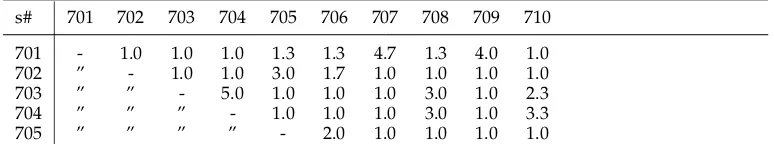
In the Usim annotation (Erk, McCarthy, and Gaylord 2009, 2013), annotators saw a pair of sentences at a time that both contained an instance of the same target word. Annotators then provided a graded judgment on a scale of 1–5 of how similar the usage of the target lemma was in the two sentences. Multiple annotators rated each sentence pair. Table 3 shows the average judgments for thepost.nexample between each pair of sentence ids in Table 1.4

3 We usen,v,a,rsuffixes to denote nouns, verbs, adjectives, and adverbs, respectively.

Table 2

Paraphrases and translations for sentences with the lemmapost.nfrom theLEXSUBandCLLS data. The same sentences were used to elicit both substitute sets.

s# LEXSUB CLLS

701 position 3; job 2; role 1; puesto 2; cargo 1; posicion 1; anuncio 1; 702 mail 2; postal service 1; date 1; post office 1; enviado 1; mostrando 1; publicado 1; saliendo

1; anuncio 1; correo 1; marcado por correo 1; 703 pole 3; support 2; stake 1; upright 1; poste 3; cerco 1; colocando 1; desplegando 1; 704 support 2; pole 2; stake 2; upright 1; poste 3; cerco 1; tabla 1;

705 mail 4; mail carrier 1; correo 2; posicion 1; puesto 1; publication 1;_{anuncio 1;} 706 message 2; electronic mail 1; mail 1;_{announcement 1; electronic bulletin 1;} entrada 4;

707 position 3; the job 2; employment 1; job 1; puesto3; cargo 2; posicion 1; publicacion 1; oficina 1;

708 support 2; marker 1; target 1; pole 1;_{boundary 1; upright 1;} poste 3;

709 position 3; job 2; appointment 1; situation 1;_{role 1;} puesto 3; posicion 2; cargo 1; anuncio 1; 710 _{crossing 3; station 2; lookout 1; fence 1;} caseta 2; puesto fronterizo 1; poste 1; correo 1;

frontera 1; cerco 1; puesto 1; caseta fronteriza 1;

The three data sets overlap in the sentences that they cover: Both Usim andCLLSare drawn from a subset of the data fromLEXSUB.5The overlap between all three data sets is 45 lemmas each in the context of ten sentences.6In this article we only use data from this common subset as it provides us with a gold-standard (Usim) and two different representations of the instances (LEXSUBandCLLSsubstitutes). The 45 lemmas in this subset include 14 nouns, 14 adjectives, 15 verbs, and 2 adverbs.7

In our experiments herein, we use the Usim data as a gold-standard of how difficult to partition usages of a lemma is. We use both LEXSUB and CLLS independently as the basis for intra-clust clusterability experiments. We compare clusterings based on LEXSUBandCLLSfor the inter-clust clusterability experiments.

3. Measuring Clusterability

We present two main approaches to estimating clusterability of word usages using the translation and paraphrase data from CLLS and LEXSUB. Firstly, we estimate cluster-ability using intra-clust measures from machine learning. Secondly, our inter-clust

5 Some sentences inLEXSUBdid not have two or more responses and for that reason were omitted from the data.

6 Usim data were collected in two rounds. For the four lemmas where there is both round 1 and round 2 Usim andCLLSdata, we use round 2 data only because there are more annotators (8 for round 2 in contrast to 3 for round 1) (Erk, McCarthy, and Gaylord 2013).

Table 3

Average Usim judgments forpost.n.

s# 701 702 703 704 705 706 707 708 709 710

701 - 1.0 1.0 1.0 1.3 1.3 4.7 1.3 4.0 1.0

702 ” - 1.0 1.0 3.0 1.7 1.0 1.0 1.0 1.0

703 ” ” - 5.0 1.0 1.0 1.0 3.0 1.0 2.3

704 ” ” ” - 1.0 1.0 1.0 3.0 1.0 3.3

705 ” ” ” ” - 2.0 1.0 1.0 1.0 1.0

method uses clustering evaluation metrics to compare agreement between two cluster-ings obtained fromCLLSandLEXSUBbased on the intuition that less clusterable lemmas will have lower congruence between solutions from the two data sets (which provide different views of the same underlying data).

3.1 Intra-Clustering Clusterability Measures

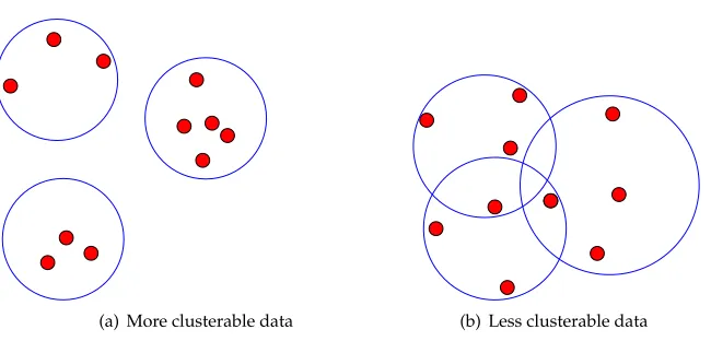
The notion of the general clusterability of a data set (as opposed to the goodness of any particular clustering) is explored within the field of machine learning by Ackerman and Ben-David (2009a). Consider for example the plots in Figure 1, where the data points on the left should be more clusterable than those on the right because the partitions are easier to make. All the notions of clusterability that Ackerman and Ben-David consider are based onk-means and involve optimum clusterings for a fixedk.

We consider three measures of clusterability that all assume ak-means clustering. LetXbe a set of data points, then ak-meansk-clustering ofXis a partitioning ofXinto ksets. We writeC={X1,. . .,Xk}for ak-clustering ofX, withSki=1Xi=X. Thek-means

loss function for ak-clusteringCis the sum of squared distances of all data points from the centroid of their cluster,

L(C)=

k

X

i=1 X

x∈Xi

||x−centroid(Xi)||2 (1)

(a) More clusterable data (b) Less clusterable data

Figure 1

where the centroid or center mass of a setYof points is

centroid(Y)= 1

|Y|

X

y∈Y

y (2)

A “k-means optimalk-clustering” of the setXis ak-clustering ofXthat has the minimal k-means loss of allk-clusterings ofX. There may be multiple such clusterings.

The first measure of clusterability that we consider isvariance ratio(VR), introduced by Zhang (2001). Its underlying intuition is that in a good clustering, points should be close to the centroid of their cluster, and clusters should be far apart. For a set Yof points,

σ2(Y)= 1

|Y|

X

y∈Y

||y−centroid(Y)||2 ₍₃₎

is the variance ofY. For ak-clusteringC ofX, we write pi= ||XXi||, and define within-cluster varianceW(C) and between-cluster varianceB(C) ofCas follows:

W(C) = Pk

i=1piσ2(Xi)

B(C) = Pk

i=1pi||centroid(Xi)−centroid(X)||2

(4)

Then the variance ratio of the data setXfor the numberkof clusters is

VR(X,k)=max

C∈Ck

B(C)

W(C) (5)

whereCkis the set ofk-means optimalk-clusterings ofX. A higher variance ratio

indi-cates better clusterability because variance ratio rises as the distance between clusters increases (B(C)) and the distance within clusters decreases (W(C)).

Worst pair ratio (WPR) uses a similar intuition as variance ratio, in that it, too, considers a ratio of a within-cluster measure and a between-cluster measure. But it focuses on “worst pairs” (Epter, Krishnamoorthy, and Zaki 1999), the closest pair of points that are in different clusters, and the most distant points that are in the same cluster. For two data pointsx,y∈Xand ak-clusteringCofX, we writex∼_Cyifxand yare in the same cluster ofC, andx6∼_Cyotherwise. Then the split ofCis the minimum distance of two data points in different clusters, and the width ofCis the maximum distance of two data points in the same cluster:

split(C) = minx,y∈X,x6∼Cy||x−y||

width(C) = maxx,y∈X,x∼Cy||x−y||

(6)

We use the variant of worst pair ratio given by Ackerman and Ben-David (2009b), as their definition is analogous to variance ratio:

WPR(X,k)=max

C∈Ck

split(C)

whereCkis the set ofk-means optimalk-clusterings ofX. Worst pair ratio is similar to

variance ratio but can be expected to be more affected by noise in the data, as it only looks at two pairs of data points while variance ratio averages over all data points.

The third clusterability measure that we use is separability (SEP), due to Ostrovsky et al. (2006). Its intuition is different from that of variance ratio and worst pair ratio: It measures the improvement in clustering (in terms of the k-means loss function) when we move from (k−1) clusters to k clusters. We write Opt_k(X)=

minC k-clustering ofXL(C) for thek-means loss of ak-means optimalk-clustering ofX. Then

a data setXis (k,ε) separable if Opt_k(X)≤εOpt_k−1(X). Separability-based clusterabil-ity is defined by

SEP(X,k)= the smallestεsuch that

Xis (k,ε)-separable (8)

Whereas for variance ratio and worst pair ratio higher values indicate better cluster-ability, the opposite is true for separability: Lower values of separability signal a larger drop ink-means loss when moving from (k−1) tokclusters.8

The clusterability measures that we describe here all rely on k-means optimal clusterings, as they were all designed to prove properties of clusterings in the area of clustering theory. To use them to test clusterability of concrete data sets in practice, we use an external measure to determinek(described in Section 4.3), and we approx-imate k-means optimality by performing many clusterings of the same data set with different random starting points, and using the clustering with minimalk-means loss L.

3.2 Inter-Clustering Clusterability Measures

If the instances of a lemma are highly clusterable, then an instance clustering derived from monolingual paraphrase substitutes and a second clustering of the same instances derived from translation substitutes should be relatively similar. We compare two clus-tering solutions using the SemEval 2010 WSItask (Manandhar et al. 2010) measures: V-measure (V) (Rosenberg and Hirschberg 2007) and paired F score (pF) (Artiles, Amig ´o, and Gonzalo 2009).

V is the harmonic mean of homogeneity and completeness. Homogeneity refers to the degree that each cluster consists of data points primarily belonging to a single gold-standard class, and completeness refers to the degree that each gold-standard class consists of data points primarily assigned to a single cluster. TheVmeasure is noted to depend on both entropy and number of clusters: Systems that provide more clusters do better. For this reason, Manandhar et al. (2010) also used the paired F score (pF), which is the harmonic mean of precision and recall. Precision is the number of common instance pairs between clustering solution and gold-standard classes divided by the number of pairs in the clustering solution, and recall is the same numerator but divided by the total

number of pairs in the gold-standard.pFpenalizes a difference in number of clusters to the gold-standard in either direction.9

4. Experimental Design

In our experiments reported here, we test both intra-clust and inter-clust clusterability measures. All clusterability results are computed on the basis of LEXSUB and CLLS data. The clusterings that we use for the intra-clust measures arek-means clusterings. We usek-means because this is how these measures have been defined in the machine learning literature; ask-means is a widely used clustering, this is not an onerous restric-tion. The similarity between sentences used byk-means is defined in Section 4.2. The k-means method needs the numberkof clusters as input; we determine this number for each lemma by a simple graph-partitioning method that groups all instances that have a minimum number of substitutes in common (Section 4.3). The graph-partitioning method is also used for the inter-clust approach, since it provides the simplest partition-ing of the data and determines the number of partitions (clusters) automatically.

In addition to the intra-clust and inter-clust clusterability measures, we test a base-line measure based on degree of overlap in an overlapping clustering (Section 4.4).

We compare the clusterability ratings to two gold standard partitionability esti-mates, both of which are derived from Usim (Section 4.1). We perform two experiments to measure how well clusterability tracks partitionability (Section 4.6).

4.1 The Gold Standard: Estimating Partitionability from Usim

We turn Usim data into partitionability information in two ways. First, we model partitionability as inter-tagger agreement on Usim (Uiaa): Uiaa is the inter-tagger agreement for a given lemma taken as the average pairwise Spearman’s correlation between the ranked judgments of the annotators. Second, we model partitionability through the proportion of mid-range judgments over all instances for a lemma and all annotators (Umid). We follow McCarthy (2011) in calculating Umid as follows. Mid-range judgments are between 2 and 4, that is not 1 (completely different usages) and not 5 (the same usage). Leta∈Abe an annotator from the setAof all annotators, and ja∈Plbe the judgment of annotatorafor a sentence pair for a lemma from all possible

such pairings for that lemma (Pl). Then the Umid score for that lemma is calculated as

Umid=

P

a∈A

P

ja∈Pl1if ja∈ {2, 3, 4}

|A| · |Pl|

(9)

Umid is a more direct indication of partitionability than Uiaa in that one might have high values of inter-tagger agreement where annotators all agree on mid-range scores. Uiaa is useful as it demonstrates clearly that these measures can indicate “tricky” lem-mas that might prove problematic for human annotators and computational linguistic systems.

4.2 Similarity of Sentences ThroughLEXSUBandCLLSfork-Means Clustering

The LEXSUB data for a sentence, for example, an instance of post.n, is turned into a vector as follows. Each possible LEXSUBsubstitute for post.nover all its ten instances becomes a dimension. For a given sentence, for example sentence 701 in Table 2, the value for dimensiontis the number of timestwas named as a substitute for sentence 701. So the vector for sentence 701 has an entry of 3 in the dimensionposition, an entry of 2 in the dimensionjob, and a value of 1 in the dimensionrole, and zero in all other dimensions, and analogously for the other instances. TheCLLSdata is turned into one vector per instance in the same way. This results in vectors of the same dimensionality for all instances of the same lemma, though the instances of different lemmas can be in different spaces (which does not matter, as they will never be compared). The distance (dvec) between two instances s,s0 of the same lemma` is calculated as the Euclidean

distance between their vectors. If there are n substitutes overall for ` across all its instances, then the distance ofsands0is

dvec(s,s0)=

v u u t

n

X

i=1

(si−s0i)2 (10)

4.3 Graphical Partitioning

This subsection describes the method that we use for determining the number of clus-ters (k) for a given lemma needed by the intra-clust approach described in Section 3.1, and for providing data partitions for the inter-clust measure of clusterability described in Section 3.2. We adopt a simple graph-based approach to partitioning word usages according to their distance, following Di Marco and Navigli (2013). Traditionally, graph-based WSI algorithms reveal a word’s senses by partitioning a co-occurrence graph built from its contexts into vertex sets that group semantically related words (V´eronis 2004). In these experiments we build graphs for the LEXSUB and CLLStarget lemmas and partition them based on the distance of the instances, reflected in the substitute annotations. Although the graphical approach is straightforward and representative of the sort of WSImethods used in our field, the exact graph partitioning method is not being evaluated here. Other graph partitioning or clustering algorithms could equally be used.

For a given lemmal, we build two undirected graphs using theLEXSUBandCLLS substitutes forl. An instance oflis identified by a sentence id (s#) and is represented by a vertex in the graph. Each instance is associated with a set of substitutes (from either LEXSUBorCLLS) as shown in Table 2 for the nounpost. Two vertices are linked by an edge if their distance is found to be low enough.

The graph partitioning method that we describe here uses a different and sim-pler estimate of distance than the k-means clustering. The distance of two vertices is estimated based on the overlap of their substitute sets. As the number of substi-tutes in each set varies, we use the size of the whole sets along with the size of the intersection for calculating the distance. Let s be an instance (sentence) from a data set (LEXSUB or CLLS) and T be the set of substitute types10 _{provided for that}

10 We have not used the frequency of each substitute, which is the number of annotators that provided it in

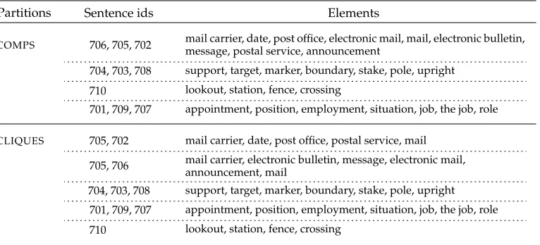
Table 4

Hard and overlapping partitions (COMPSandCLIQUES) obtained forpost.nfrom theLEXSUBdata.

Partitions Sentence ids Elements

COMPS 706, 705, 702 mail carrier, date, post office, electronic mail, mail, electronic bulletin,_{message, postal service, announcement} 704, 703, 708 support, target, marker, boundary, stake, pole, upright

710 lookout, station, fence, crossing

701, 709, 707 appointment, position, employment, situation, job, the job, role

CLIQUES 705, 702 mail carrier, date, post office, postal service, mail 705, 706 mail carrier, electronic bulletin, message, electronic mail,

announcement, mail

704, 703, 708 support, target, marker, boundary, stake, pole, upright 701, 709, 707 appointment, position, employment, situation, job, the job, role 710 lookout, station, fence, crossing

instance inLEXSUB orCLLS. The distance (dnode) between two instances (nodes)sand

s0with substitute setsTandT0corresponds to the number of moves necessary to convert TintoT0. We use the metric proposed by Goldberg, Hayvanovych, and Magdon-Ismail (2010), which considers the elements that are shared by, and are unique to, each of the sets.

dnode(T,T0)=|T|+|T0| −2|T∩T0| (11)

We consider two instances as similar enough to be linked by an edge if their intersection is not empty (i.e., they have at least one common substitute) and their distance is below a threshold. After observation of the distance results for different lemmas, the threshold was defined to be equal to 7.11A pair of instances with a distance below the threshold is linked by an edge in the graph. For example, instances 705 and 706 ofpost.nare linked in the graph built from theLEXSUBdata (cf. Table 2) because their intersection is not empty (they sharemail) and they have a distance of 5. The graph built for a lemma is partitioned into connected components (hereafterCOMP). As the COMPSdo not share any instances, they correspond to a hard (non-overlapping) clustering solution over the set of instances. Two instances belong to the same component if there is a path between their vertices. The top part of Table 4 displays theCOMPSobtained forpost.nfrom the LEXSUBdata. The 10 instances of the lemma in Table 2 are grouped into four COMPS. Instances 705 and 706 that were linked in the graph are found in the same connected component. On the contrary, 710 shares no substitutes with any other instance as shown in Table 2, and, as a consequence, does not satisfy either the intersection or the distance criterion. Instance 710 is thus isolated as it is linked to no other instances, and forms a separate component.

1 2 3 4 5 7 8 CLLS LEXSUB

number of COMPS

freq

0

5

10

15

Figure 2

Frequency distribution over number ofCOMPS: How many lemmas had a given number of COMPSin the two data sets.

Figure 2 shows the frequency distribution of lemmas over number ofCOMPS.

4.4 A Baseline Measure Based on Cluster Overlap

Our proposed clusterability measures (both intra- and inter-clust) are applicable to hard clusterings.WSIin computational linguistics has traditionally focused on a hard partition of usages into senses but there have been recent attempts to allow for graded annotation (Erk, McCarthy, and Gaylord 2009, 2013) and soft clustering (Jurgens and Klapaftis 2013). We wanted to see how well the extent of overlap between clusters might be used as a measure of clusterability because this information is present for any soft clustering. If this simple criterion worked well, it would avoid the need for an independent measure of clusterability. If the amount of overlap is an indicator of clusterability then soft clustering can be applied and lemmas with clear-cut sense distinctions will be identified as having little or no overlap between clusters, as depicted in Figure 3.

For this baseline, we measure overlap from a second set of node groupings of the graphs described in Section 4.3, where an instance can fall into more than one of the groups. We refer to this soft grouping solution as CLIQUES. A clique consists of a

(a) More clusterable data (b) Less clusterable data

Figure 3

Data Graph partitioning Clusterability metric

LexSub

CLLS

comps

Parameter definition

intra-clustering (VR, SEP, WPR)

cliques

comps

cliques

k

baseline (ncs)

inter-clustering (pf, V) baseline (ncs)

k intra-clustering (VR, SEP, WPR)

Figure 4

Illustration of the processing pipeline from input data to clusterability estimation.

maximal set of nodes that are pairwise adjacent.12_{They are typically finer grained than} theCOMPSbecause there may be vertices in a component that have a path between them without being adjacent.13

The lower part of Table 4 contains theCLIQUESobtained forpost.ninLEXSUB. The two solutions, COMPS and CLIQUES, presented for the lemma in this table are very similar except that there is a further distinction in theCLIQUES as the first cluster in theCOMPSis subdivided between two different senses ofmail(broadly speaking, the

physical and electronic senses). Note that these two CLIQUES overlap and share

instance 705.

We wish to see if using the extent of overlap in the CLIQUESreflects the partition-ability numbers derived from the Usim data to the same extent as the clusterpartition-ability metrics already presented. If it does, then the overlapping clustering approach itself could be used to determine how easily the senses partition and clusterability would be reflected by the extent of instance overlap in the clustering solution. LetCsbe the set of

partitions (CLIQUES) to which a sentencesfrom the sentences for a given lemma (Sl) is

automatically assigned. Thenncs(l) measures the average number ofCLIQUESto which

the sentences for a given lemma are assigned.

ncs(l)=

P

s∈Sl|Cs|

|Sl| (12)

We assume that lemmas that are less easy to partition will have higher values ofncs

compared with lemmas with a similar number of clusters over all sentences but with lower values ofncs.

4.5 Experimental Design Overview

In Figure 4 we give an overview of the whole processing pipeline, from the input data to the clusterability estimation. The graphs built for each lemma from theLEXSUBandCLLS

12 Cliques are computed directly from a graph, not from theCOMPS.

Table 5

Overview of gold partitionability estimates and of clusterability measures to be evaluated.

Gold partitionability estimates Umid: proportion of mid-range (2–4) instance similarity ratings for a lemma

Uiaa: inter-annotator agreement on the Usim data set (average pairwise Spearman)

Intra-clust clusterability measures VR,WPR,SEPbased onk-means clustering

kestimated asCOMPS

clustering computed based on either LEXSUB or CLLS substitutes

Inter-clust clusterability measures comparing COMPS partitioning of CLLS with COMPS partitioning ofLEXSUB

comparison either throughVorpF

Baseline average numberncsofCLIQUESclusters, computed either fromLEXSUBorCLLSdata

data are partitioned twice creating COMPS and CLIQUES. The COMPSserve to define the kper lemma needed by the intra-clust clusterability metrics (VR, SEP, WPR). The inter-clust metrics (VandpF) compare the two sets ofCOMPScreated for a lemma from the LEXSUBand CLLSdata. The overlaps present in theCLIQUESare exploited by the baseline metric (ncs).

4.6 Evaluation

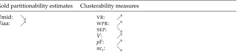
Table 5 provides a summary of the two gold standard partitionability estimates and the two types of clusterability measures, along with the baseline clusterability measure that we test. The partitionability estimates and the clusterability measures vary in their directions: In some cases, high values denote high partitionability; in other cases high values indicate low partitionability. Because WPR and VR are predicted to have high values for more clusterable lemmas andSEPhas low values, we expectWPRandVRto positively correlate with Uiaa and negatively with Umid and the direction of correlation to be reversed for SEP. Our clustering evaluation metrics (V and pF) should provide correlations with the gold standards in the same direction asWPRandVRsince a high congruence between the two solutions for a lemma from different annotations of the same sentences should be indicative of higher clusterability and consequently higher values of Uiaa and lower values of Umid. As regards the baseline approach based on cluster overlap, because we assume that lemmas that are less easy to partition will have higher values ofncs, high values ofncsshould be positively correlated with Umid and

negatively correlated with Uiaa (like SEP). Table 6 gives an overview of the expected directions.

Table 6

Directions of partitionability estimates and clusterability measures:%means that high values denote high partitionability, and&means that a high value denotes low partitionability.

Gold partitionability estimates Clusterability measures

Umid: & VR: %

Uiaa: % WPR: %

SEP: &

V: %

pF: %

ncs: &

decreases as the number of clusters rises (this affects the within-cluster varianceW(C) and width(C)). Separability is always lowest for k=n (number of data points), and almost always second-lowest fork=n−1.

The first set of experiments measures correlation using Spearman’s ρ between a ranking of partitionability estimates and a ranking of clusterability predictions. We do not perform correlation across all lemmas but control for polysemy by grouping lemmas into polysemy bands, and performing correlations only on lemmas with a polysemy within the bounds of the same band. Letkbe the number of clusters for lemmal, which is the number ofCOMPSfor all clusterability metrics other thanncs, and the number of

CLIQUESfor ncs. For the cluster congruence metrics (Vand pF), we take the average

number of clusters for a lemma in both LEXSUB and CLLS.14 Then we define three polysemy bands:

r

r

r

Note that none of the intra-clust clusterability measures are applicable for k=1, so in cases where the number ofCOMPSis one, the lemma is excluded from analysis. In these cases the clustering algorithm itself decides that the instances are not easy to partition.

The second set of experiments performs linear regression to link partitionability to clusterability, using the degree of polysemyk as an additional independent variable. As we expect polysemy to interfere with all clusterability measures, we are interested not so much in polysemy as a separate variable but in the interaction polysemy ×

clusterability. This lets us test experimentally whether our prediction that polysemy influences clusterability is borne out in the data. As the second set of experiments does not break the lemmas into polysemy bands, we have a single, larger set of data points undergoing analysis, which gives us a stronger basis for assessing significance.

5. Experiments

In this section we provide our main results evaluating the various clusterability mea-sures against our gold-standard estimates. Section 5.1 discusses the evaluation via correlation with Spearman’s ρ. In Section 5.2 we present the regression experiments. In Section 5.3 we provide examples and lemma rankings by two of our best performing metrics.

5.1 Correlation of Clusterability Measures Using Spearman’sρ

We calculated Spearman’s correlation coefficient (ρ) for both gold standards (Uiaa and Umid) against all clusterability measures: intra-clust (VR,WPR, andSEP), inter-clust (V andpF), and the baselinencs. For all these measures except the inter-clust, we calculate

ρusingLEXSUBandCLLSseparately as our clusterability measure input. The inter-clust measures rely on two views of the data so we useLEXSUBandCLLStogether as input. We calculate the correlation for lemmas in the polysemy bands (low, mid, and high, as described above in Section 4.6) subject to the constraint that there are at least five lemmas within the polysemy range for that band. We provide the details of all trials in Appendix A and report the main findings here.

Table 7 shows the average Spearman’sρover all trials for each clusterability mea-sure. Although there are a few non-significant results from individual trials that are in the unanticipated direction (as discussed in the following paragraph), all averageρare in the anticipated direction, specified in Table 6; SEPand ncs are positively correlated

with Umid and negatively with Uiaa whereas for all other measures the direction of correlation is reversed. Some of the metrics show a promising level of correlation but the performance of the metrics varies. The baselinencsis particularly weak, highlighting

that the amount of shared sentences in overlapping clusters is not a strong indication of clusterability. This is important because if this simple baseline had been a good indicator of clusterability, then a sensible approach to the phenomenon of partionability of word meaning would be to simply soft cluster a word’s instances and the extent of overlap would be a direct indication that the meanings are highly intertwined.WPRis also quite

Table 7

The macro-averaged correlation of each clusterability metric with the Usim gold-standard rankings Uiaa and Umid: All correlations are in the expected direction. Also, the proportion (prop.) of trials from Tables A.1–A.5 in Appendix A with moderate or stronger correlation in the correct direction with a statistically significant result.

measure averageρ prop.ρ >0.4* or **

type measure Umid Uiaa Umid Uiaa

intra-clust

VR −0.483 0.365 2/3 2/3

SEP 0.569 −0.390 2/3 1/3

WPR −0.322 0.210 1/3 0/3

inter-clust pF_V −₋0.318_0.123 0.540_0.493 0/2_0/2 1/2_0/2

weak, which is not unexpected: It only considers the worst pair rather than all data points, as noted in Section 3.1. Both inter-clust measures (pF andV) have a stronger correlation with Uiaa than with Umid, whereas for the machine learning measures the reverse is true and the correlation is stronger for Umid. As mentioned in Section 4.1, Umid is a more direct gold-standard indicator of partitionability but Uiaa is useful as a gold standard as it indicates how problematic annotation will be for humans. The machine learning metricSEPand our proposal forpFas an indication of clusterability provide the strongest average correlations, though the results forpFare less consistent over trials.15

Because we are controlling for polysemy, there is less data (lemmas) for each cor-relation measurement so many individual trials do not give significant results, but all significant correlations are in the anticipated direction. The final two columns of Table 7 show the proportion of cases that are significant at the 0.05 level or above and have

ρ >0.416 _{in the anticipated direction out of all individual trials meeting the constraint} of five or more lemmas in the respective polysemy band forLEXSUBorCLLSinput data. We are limited by the available gold-standard data and need to control for polysemy. So there are several results with a promisingρwhich, however, are not significant, such that they are scored negatively in this more stringent summary. Nevertheless, from this summary of the results we can see that the machine learning metrics, particularlyVR (which has a higher proportion of successful trials) and SEP (which has the highest average correlations) are most consistent in indicating partitionability using either gold-standard estimate (Umid or Uiaa) withVR achieving 66.7% success (2 out of 3 trials for each gold-standard ranking).WPR is less promising for the reasons stated above. Although there are some successful trials for the inter-clust approaches, the results are not consistent and only one trial showed a (highly) significant correlation. The baseline approach which measures cluster overlap has only one significant result in all 6 trials, but more worrisome for this measure is the fact that in 4 out of the 12 trials (2 for each Umid and Uiaa) the correlation was in the non-anticipated direction. In contrast there was only one result forWPR(onCLLS) in the non-anticipated direction and one result forV on the fence (ρ=0) and all other individual results for the inter and intra-clust measures were in the anticipated direction.

There were typically more lemmas in the intra-clust trials withLEXSUBcompared to CLLS, as shown in Appendix A due to the fact that many lemmas inCLLShave only one component (see Figure 2) and are therefore excluded from the intra-clust clusterability estimation.17

5.2 Linking Partitionability to Clusterability and Polysemy Through Regression

Our first round of experiments revealed some clear differences between approaches and implied good performance, particularly for the intra-clust measuresVRandSEP. In the first round of experiments, however, we separated lemmas into polysemy bands and this resulted in the set of lemmas involved in each individual correlation experiment being somewhat small. This makes it hard to obtain significant results. Even for the

15 This can be seen in Table A.3 in Appendix A.

16 This is generally considered the lower bound of moderate correlation for Spearman’s and is the level of inter-annotator agreement achieved in other semantics tasks (for example see Mitchell and Lapata [2008]).

overall most successful measures, not all trials came out as significant. In this second round of experiments, we therefore change the set-up in a way that allows us to test on all lemmas in a single experiment, to see which clusterability measures will exhibit an overall significant ability to predict partitionability.

We use linear regression, an analysis closely related to correlation.18The dependent variable to be predicted is a partitionability estimate, either Umid or Uiaa. We use two types of independent variables (predictors). The first is the clusterability measure— here we call this variable clust. The second is the degree of polysemy, which we call poly. This way we can model an influence of polysemy on clusterability as an interaction of variables, and have all lemmas undergo analysis at the same time. This lets us obtain more reliable results: Previously, a non-significant result could indicate either a weak predictor or a data set that was too small after controlling for poly-semy, but now the data set undergoing analysis is much bigger.19 _{Furthermore, this} experiment demonstrates how clusterability and polysemy can be used together as predictors.

The variable clust reflects the clusterability predictions of each measure. We use the actual values, not their rank among the clusterability values for all lemmas. This way we can test the ability of our clusterability measures to predict partitionability for individual lemmas, while the rank is always relative to other lemmas that are being analyzed at the same time. The values of the variable clust are obviously dif-ferent for each clusterability measure, but the values of poly also vary across clus-terability measures: For all intra-clust measures poly is the number of COMPS. For the inter-clust measures, it is the average number of COMPS between the numbers computed from LEXSUB and from CLLS. For the ncs baseline it is the number of

CLIQUES. In all cases, poly is the actual number ofCOMPSorCLIQUES, not the polysemy band.

We test three different models in our linear regression experiment. The first model has poly as its sole predictor. It tests to what extent partitionability issues can be explained solely by a larger number of COMPS or CLIQUES. Our hypothesis is that this simple model will not suffice. The second model has clust as its sole predictor, ignoring possible influences from polysemy. The third model uses the in-teraction poly × clust as a predictor (along with poly and clust as separate vari-ables). Our hypothesis is that this third model should fare particularly well, given the influence of polysemy on clusterability measures that we derived theoretically above.20

We evaluate the linear regression models in two ways. The first is the F test. Given a model M predicting Y from predictors X1,. . .,Xm as Y=β0+β1X1+. . .+βmXm,

it tests the null hypothesis thatβ₀ =β₁=. . .=β_m =0. That is, it tests whetherMis statistically indistinguishable from a model with no predictors.21 _{Second, we use the} Akaike Information Criterion (AIC) to compare models. AIC tests how well a model

18 The regression coefficient is a standardization of Pearson’s r, a correlation coefficient, related via a ratio of standard deviations.

19 Also, the first round of experiments had to drop some lemmas from the analysis when they were in a polysemy band with too few members; the second round of experiments does not have this

issue.

20 We also tested a model with predictors poly+clust, without interaction. We do not report on results for this model here as it did not yield any interesting results. It was basically always between clust and poly×clust.

Table 8

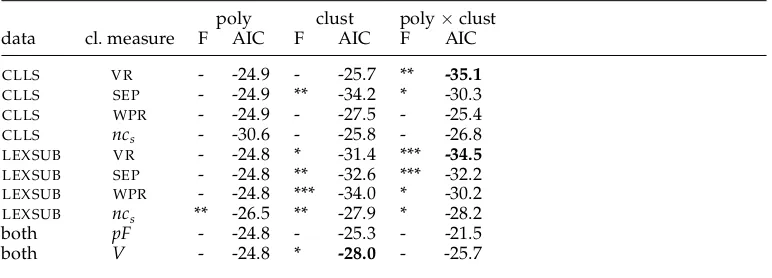
Regression results for theUmid partitionability estimate. Significance of F statistic, and AIC for the following models: polysemy only (poly), clusterability only (clust), and interaction (poly×clust).Bolded: model that is best by AIC and has significant F, separately for each substitute set. We use * for statistical significance with p<0.05, ** for p<0.01, and *** for p<0.001.

poly clust poly×clust

data cl. measure F AIC F AIC F AIC

CLLS VR - -24.9 - -25.7 ** -35.1

CLLS SEP - -24.9 ** -34.2 * -30.3

CLLS WPR - -24.9 - -27.5 - -25.4

CLLS ncs - -30.6 - -25.8 - -26.8

LEXSUB VR - -24.8 * -31.4 *** -34.5

LEXSUB SEP - -24.8 ** -32.6 *** -32.2

LEXSUB WPR - -24.8 *** -34.0 * -30.2

LEXSUB ncs ** -26.5 ** -27.9 * -28.2

both pF - -24.8 - -25.3 - -21.5

both V - -24.8 * -28.0 - -25.7

will likely generalize (rather than overfit) by penalizing models with more predictors. AIC uses the log likelihood of the model under the data, corrected for model complexity computed as its number of predictors. Given again a modelMpredictingY(in our case, either Umid or Uiaa) frommpredictors, the AIC is

AIC=−2 logp(Y|M)+2m

The lower the AIC value, the better the generalization of the model. The model preferred by AIC is the one that minimizes the Kullback-Leibler divergence between the model and the data. AIC allows us to compare all models that model the same data, that is, all models predicting Umid can be compared to each other, and likewise all models predicting Uiaa.

The number of data points in each model depends on the partitioning (as lemmas withk=1 cannot enter into intra-clust clusterability analysis), which differs between CLLSandLEXSUB. AIC depends on the sample size (throughp(Y|M)), so in order to be able to compare all models that model the same partitionability estimate, we compute AIC only on the subset of lemmas that enters in all analyses.22_{In contrast, we compute} the F test on all lemmas where the clusterability measure is valid,23_{in order to use the} largest possible set of lemmas to test the viability of a model.24

Table 8 shows the results for models predicting Umid, and Table 9 shows the results for the prediction of Uiaa. The bolded figures are the best AIC values for each substitute set (CLLS,LEXSUB, both) where the corresponding F-tests reach significance.25

22 This subset comprises 27 lemmas: charge.v, clear.v, draw.v, dry.a, fire.v, flat.a, hard.r, heavy.a, hold.v, lead.n, light.a, match.n, paper.n, post.n, range.n, raw.a, right.r, ring.n, rude.a, shade.n, shed.v, skip.v, soft.a, solid.a, stiff.a, tap.v, throw.v.

23 For the intra-clust measures, this is only lemmas wherek>1.

24 We also computed AIC separately for substitute setsLEXSUB,CLLS, and both (for inter-clust). The relative ordering of models within each substitute set remained mostly the same.

Table 9

Regression results for theUiaa partitionability estimate. Significance of F statistic, and AIC for the following models: polysemy only (poly), clusterability only (clust), and interaction (poly×clust). Bolded: model that is best by AIC and has significant F, separately for each substitute set. We use * for statistical significance with p<0.05 and ** for p<0.01.

poly clust poly×clust

data cl. measure F AIC F AIC F AIC

CLLS VR - -20.2 - -21.2 - -20.7

CLLS SEP - -20.2 - -23.0 - -20.9

CLLS WPR - -20.2 - -24.1 - -21.8

CLLS ncs - -20.8 - -20.3 - -19.3

LEXSUB VR - -20.4 - -21.7 * -26.9

LEXSUB SEP - -20.4 ** -27.7 * -25.4

LEXSUB WPR - -20.4 * -29.7 - -27.0

LEXSUB ncs - -22.7 ** -21.4 ** -24.8

both pF - -20.0 - -22.1 - -18.8

both V - -20.0 - -24.8 - -21.9

Confirming the results from our first round of experiments, we obtain the best results forSEPandVR: The best AIC results in predicting Umid are reached byVR, while SEPshows a particularly reliable performance. In predicting Umid, allSEPmodels that use clust reach significance, and in predicting Uiaa, allSEPmodels that use clust reach significance if they are based on LEXSUBsubstitutes.WPRreaches the best AIC values on predicting Uiaa, but on the F test, which takes into account more lemmas, its results are less often significant.

As in the first round of experiments, the performance of the two inter-clust mea-sures is not as strong as that of the intra-clust meamea-sures. Here the inter-clust meamea-sures are in fact often comparable to thencsbaseline. However, asCLLSseems to be harder to

use as a basis thanLEXSUB(we comment on this subsequently), the inter-clust measures may be hampered by problems with theCLLSdata.

The baselinencs measure does not have as dismal a performance here as it did in

the first round of experiments, but its performance is still worse throughout than that of the intra-clust measures. Interestingly, the poly variable that we use forncs, which is the

absolute number ofCLIQUESfor a lemma, is informative to some extent for Umid but not for Uiaa, and the clust variable is informative to some extent for Uiaa but not for Umid.

The regression experiments overall confirm the influence of polysemy on the clus-terability measures. Although clusclus-terability as a predictor on its own (the clust models) often reaches significance in predicting partitionability, taking polysemy into account (in the poly × clust models) often strengthens the model in predicting Umid and achieves the overall best results (the two bolded models); however for Uiaa the results are more ambivalent, where of the four clusterability measures that produce significant models, two improve when the interaction with polysemy is taken into account, and the two others do not. We also note thatCOMPSalone (the poly variable for the intra-clust models) never manages to predict partitionability in any way, for either Umid or Uiaa. In contrast, the number of CLIQUES(the poly variable of thencs model) emerges as a

predictor of Umid, though not of Uiaa.

Comparing theCLLSandLEXSUBsubstitutions, we see that the use ofLEXSUBleads to much better predictions than CLLS. Most strikingly, in predicting Uiaa no model achieves significance usingCLLS. We have commented on this issue before: The reason for this effect is that many lemmas inCLLShave only one component and are therefore excluded from the intra-clust clusterability estimation.

Clusterability in practice.As this round of experiments used the raw clusterability figures to predict partitionability, rather than their rank, it points the way to using clusterability in practice: Given a lemma, collect instance data (for example paraphrases, translations, or vectors). Estimate the number of clusters, for example using a graphical clustering approach. Then use a clusterability measure (SEP or VR recommended) to determine its degree of clusterability, and use a regression classifier to predict a partitionability estimate. It may help to take the interaction of clust and poly into account. If the estimate is high, then a hard clustering is more likely to be appropriate, and sense tagging for training or testing should not be difficult. Where the estimate is low it is more likely that a more complex graded representation is needed, and in extreme cases clustering should be avoided altogether. Determining where the boundaries are would depend on the purpose of the lexical representation and is not addressed in this article. Our contribution is an approach to determine the relative location of lemmas on a continuum of partitionability.

5.3 Lemma Clusterability Rankings and Some Examples

Our clusterability metrics, in particular VR and SEP, are useful for determining the partitionability of lemmas. In this section we show the rankings for these two metrics with our lemmas and provide a couple of more detailed examples with theLEXSUBand CLLSdata.

In Table 10 we show the lemmas that havek>1 when partitioned intoCOMPSusing theLEXSUBsubstitutes, their respective gold standard Umid and Uiaa values, and the SEP and VR values calculated for them on the basis ofLEXSUBsubstitutes. The “L by Uiaa” and “L by Umid” columns display the lemmas reranked according to the two gold-standard estimates, and the “L byVR” and “L bySEP” columns do likewise for the VRandSEPclusterability measures. We have reversed the order of the ranking by Umid and SEP because these measures are high when clusterability is low and vice versa. Lemmas with high partitionability should therefore be near the bottom of the table in columns 7–10 and lemmas with low partitionability should be near the top. There are differences and all rankings are influenced by polysemy, but we can see from this table that on the whole the metrics rank lemmas similarly to the gold-standard rankings with highly clusterable lemmas (such asfire.v) at the bottom of the table and less clusterable lemmas (such aswork.v) nearer the top.

Table 10

Ranking of lemmas (L) by the gold-standards, and byVRandSEPforLEXSUBdata.

lemma k Umid Uiaa VR SEP L by Umid L by Uiaa L byVR L bySEP

Table 11

COMPSobtained fromLEXSUBandCLLSforfire.vandsolid.a.

LEXSUB CLLS

s# substitutes s# substitutes

fire.v

1857, 1852, 1859, 1855, 1851, 1860

discharge, shoot at, launch, shoot

1857, 1852, 1859, 1855, 1851, 1860

balear, lanzar, aparecer, prender fuego, disparar, golpear, apuntar, detonar, abrir fuego

1858, 1856,

1853, 1854 sack, dismiss, lay off

1858, 1856, 1853, 1854

correr, dejar ir, delar sin trabajo, despedir, desemplear, liquidar, dejar sin trabajo, echar, dejar sin empleo

solid.a

1081, 1083, 1087

solid, sound, set, strong, firm, rigid, dry, concrete, hard

1084

estable, solido, integro, formal, seguro, firme, real, consistente, fuerte, fundado

1090, 1082, 1088, 1085, 1084, 1089, 1086

fixed, secure, substantial, valid, reliable, good, sturdy, respectable, convincing, sound, substantive, dependable, strong, genuine, cemented, firm, accurate, stable 1090, 1081, 1087, 1086, 1082, 1083, 1085, 1088, 1089

fidedigno, con cuerpo, conciso, estable, macizo, solido, con fundamentos, tempano, fundamentado, confiable, real, seguro, firme, consistente, fuerte, estricto, congelado, en estado solido, resistente, duro, bien fundado, fundado

whereasSEPis lower as anticipated. The two lemmas were selected as examples with the same number ofCOMPSto allow for a comparison of the values. The overlap measure ncsis higher forsolid.aas anticipated.26

Note that for the highly clusterable lemmafire.vthere are no substitutes in common in the two groupings with either theLEXSUBorCLLSdata because there is no substitute overlap in the sentences, which results in the COMPS and CLIQUES solutions being equivalent, whereas forsolid.athere are several substitutes shared by the groupings for LEXSUB(e.g.,strong) andCLLS(e.g.,solido).

6. Conclusions and Future Work

In this article, we have introduced the theoretical notion of clusterability from machine learning discussed by Ackerman and Ben-David (2009a) and argued that it is relevant to WSIsince lemmas vary as to the degree of partitionability, as highlighted in the linguis-tics literature (Tuggy 1993) and supported by evidence from annotation studies (Chen and Palmer 2009; Erk, McCarthy, and Gaylord 2009, 2013). We have demonstrated here how clustering of translation or paraphrase data can be used with clusterability mea-sures to estimate how easily a word’s usages can be partitioned into discrete senses. In addition to the intra-clust measures from the machine learning literature, we have also operationalized clusterability as consistency in clustering across information sources

Table 12

Values of clusterability metrics for the examplesfire.vandsolid.a.

COMPS

LEXSUB CLLS

intra-clust fire.v solid.a fire.v solid.a

SEP 0.122 0.584 0.179 0.685

VR 7.178 0.713 4.579 0.459

WPR 1.732 0.845 1.795 0.707

LEXSUBandCLLS

inter-clust fire.v solid.a

pF 1 0.081

V 1 0.590

CLIQUES

LEXSUB CLLS

baseline fire.v(2 #cl) solid.a(4 #cl) fire.v(2 #cl) solid.a(7 #cl)

ncs 1.0 1.5 1 2.1

Gold-Standard from Usim

Gold-Standard fire.v solid.a

Uiaa 0.930 0.490

Umid 0.169 0.630

using clustering solutions from translation and paraphrase data together. We refer to this second set of measures as inter-clust measures.

We conducted two sets of experiments. In the first we controlled for polysemy by performing correlations between clusterability estimates and our gold standard on our lemmas in three polysemy bands, which allows us to look at correlation independent of polysemy. In the second set of experiments we used linear regression on the data from all lemmas together, which allows us to see how polysemy and clusterability can work together as predictors. We find that the machine learning metrics SEP and VR produce the most promising results. The inter-clust metrics (VandpF) are interesting in that they consider the congruence of different views of the same underlying usages, but although there are some promising results, the measures are not as consistent and in particular in the second set of experiments do not outperform the baseline. This may be due to their reliance on CLLS, which generally produces weaker results compared toLEXSUB. Our baseline, which measures the amount of overlap in overlap-ping clustering solutions, shows consistently weaker performance than the intra-clust measures.

Clusterability metrics should be useful in planning annotation projects (and esti-mating their costs) as well as for determining the appropriate lexical representation for a lemma. A more clusterable lemma is anticipated to be better-suited to the traditional hard-clustering winner-takes-allWSD methodology compared with a less clusterable lemma where a more complex soft-clustering approach should be considered and more time and expertise is anticipated for any annotation and verification tasks. For some tasks, it may be worthwhile to focus disambiguation efforts only on lemmas with a reasonable level of partitionability.

We believe that notions of clusterability from machine learning are particularly relevant toWSIand the field of word meaning representation in general. These notions might prove useful in other areas of computational linguistics and lexical semantics in particular. One such area to explore would be clustering predicate-argument data (Sun and Korhonen 2009; Schulte im Walde 2006).

All the metrics and gold standards measure clusterability on a continuum. We have yet to address the issue of where the cut-off points on that continuum for alternate representations might be. There is also the issue that for a given word, there may be some meanings which are distinct and others that are intertwined. It may in future be possible to find contiguous regions of the data that are clusterable, even if there are other regions where the meanings are less distinguishable.

The paraphrase and translation data we have used to examine clusterability metrics have been produced manually. In future work, the measures could be applied to auto-matically generated paraphrases and translations or to vector-space or word (or phrase) embedding representations of the instances. Use of automatically produced data would allow us to measure clusterability over a larger vocabulary and corpus of instances but we would need to find an appropriate gold standard. One option might be evidence of inter-tagger agreement from corpus annotation studies (Passonneau et al. 2012) or data on ease of word sense alignment (Eom, Dickinson, and Katz 2012).

Appendix A: Individual Spearman’s Correlation Trials

Tables A1–A5 provide the details of the individual Spearman’s correlation trials of clus-terability measures against the gold standards reported in Section 5.1. All correlations in the anticipated direction are marked inblue, and those in the counter-intuitive direction are marked inredand noted byoppin the final column. In the same column, we use * for statistical significance with p<0.05 and ** for p<0.01. We use only those polysemy bands where there are at least five lemmas within the polysemy range for that band. The number of lemmas (#) in each band is shown within parentheses.

Table A.1

Correlation of the intra-clustk-means metrics onCLLSagainst the Usim gold-standard rankings Uiaa and Umid.

Band (#) Clusterability measure Usim measure ρ sig/opp

low (22) VR Umid –0.4349 *

low (22) VR Uiaa 0.4539 *

low (22) SEP Umid 0.6077 **

low (22) SEP Uiaa –0.2041

low (22) WPR Umid –0.1187

Table A.2

Correlation of the intra-clustk-means metrics onLEXSUBwith the Usim gold-standard estimates Uiaa and Umid.

Band (#) measure1 measure2 ρ sig/opp

low (29) VR Umid –0.6058 **

mid (10) VR Umid –0.4073

low (29) VR Uiaa 0.4049 *

mid (10) VR Uiaa 0.2364

low (29) SEP Umid 0.359

mid (10) SEP Umid 0.7416 *

low (29) SEP Uiaa –0.3038

mid (10) SEP Uiaa –0.6606 *

low (29) WPR Umid –0.4161 *

mid (10) WPR Umid –0.4316

low (29) WPR Uiaa 0.2739

mid (10) WPR Uiaa 0.3818

Table A.3

Correlation of the inter-clust metrics onLEXSUB-CLLSwith the Usim gold-standards: Uiaa and Umid.

Band (#l) measure1 measure2 ρ sig/opp

low (29) pF Umid –0.1365

mid (5) pF Umid –0.5

low (29) pF Uiaa 0.1796

mid (5) pF Uiaa 0.9 *

low (29) V Umid –0.2456

mid (5) V Umid 0

low (29) V Uiaa 0.3849 *

mid (5) V Uiaa 0.6

Table A.4

Correlation of the baselinencsoperating onCLLSwith the Usim gold-standard: Uiaa and Umid.

Band (#) measure1 measure2 ρ sig/opp

low (14) ncs Umid 0.4381

mid (17) ncs Umid 0.0308

high (9) ncs Umid −0.4622 opp

low (14) ncs Uiaa −0.3455

mid (17) ncs Uiaa −0.4948 *