Applicability of Weibull Distribution to Description of Distributed Normalized Critical Current of Bent Damaged Bi2223 Composite Tape

Applicability of Weibull Distribution to Description of Distributed Normalized

Critical Current of Bent-Damaged Bi2223 Composite Tape

Shojiro Ochiai

, Hiroshi Okuda

, Michinaka Sugano

, Masaki Hojo

, Kozo Osamura

,

Tsuneo Kuroda

, Hiroaki Kumakura

, Hitoshi Kitaguchi

, Kikuo Itoh

and Hitoshi Wada

2_{Department of Electronic Science and Engineering, Kyoto University, Kyoto 615-8530, Japan} 3_{Department of Mechanical Engineering and Science, Kyoto University, Kyoto 606-8501, Japan} 4_{Research Institute for Applied Sciences, Kyoto 606-8202, Japan}

5_{Superconducting Materials Center, National Institute for Materials Science, Tsukuba 305-0047, Japan}

Critical current of bent-damaged Bi2223 composite tape differs from specimen to specimen. To describe the distributed critical current values of specimens, the three-parameter Weibull distribution function has been employed and has been demonstrated to describe the experimental results. In the present work, the reason for this was discussed by modeling analysis of the experimental results in a round robin test of VAMAS/TWA16. The distribution of the measured normalized critical current values was described well by using the damage evolution approach, in which the difference in damage evolution among the specimens was correlated to the distribution of critical current values. From this approach, the three-parameter Weibull distribution function for critical current values was derived, which gave almost the same parameter values for the minimum critical current, scale parameter and shape parameter as those obtained by the direct application of the Weibull distribution function to the experimental results. Based on this result, the reason why the normalized critical current values of bent-damaged composite tape is described by the three-parameter Weibull distribution function was accounted for in a quantitative manner by the difference in damage evolution among the specimens. [doi:10.2320/matertrans.MAW201001]

(Received March 25, 2010; Accepted June 17, 2010; Published August 4, 2010)

Keywords: Bi2223 composite superconductor, critical current distribution, bending, heterogeneous damage, Weibull distribution

1. Introduction

The critical current of Bi2223/Ag/Ag alloy composite tape under externally applied strain is known to be reduced first at the irreversible strain at which the damage of the Bi2223 filaments takes place, and then to be further reduced

with increasing strain due to damage evolution.1–14)

Hetero-geneous damage occurs, and the damage evolution behavior differs from specimen to specimen and from location to

location within a specimen.9–14)_{Accordingly, when a number}

of specimens are tested, the critical current differs from specimen to specimen.

To describe the damage-induced distribution of critical current of the bent specimens, we have recently proposed a modeling approach that incorporates the correlation among the critical current, the shape of the core where the Bi2223 filaments are embedded, the applied bending strain and the

damage evolution.11,12,14)_{In this approach, the"}

f"r value,

where"f is the fracture strain of the bare Bi2223 filaments

and "r is the residual strain of the filaments in the current

transport direction, was treated as a variable; using this value, the difference in damage amount among the specimens was

expressed. The"f"rvalue corresponds to the tensile strain

at which the filaments embedded in the composite tape are

fractured. Because the "r is negative (compressive) in the

Bi2223 composite tape, as has been demonstrated by X ray

diffraction analysis,7,8) the actual fracture strain of the

filaments in the composite tape is by "r higher than the

intrinsic fracture strain "f of the filaments alone.2,4,6–8,11,14)

The"f"rvalue is different from location to location within

a specimen as well as from specimen to specimen. In the

preceding works,11,12) the heterogeneous damage behavior

was formulated by the distributed "f"r values and was

correlated to the distribution of critical current values. The procedure for application and the features of this approach (hereinafter ‘‘damage approach’’) is presented later in Section 3.2. This approach was applied to the measured

values of the VAM1 sample in the round robin test10) _of

VAMAS (Versailles project on advanced materials and standard)/TWA 16 (Technical working area 16, supercon-ducting materials). It was shown that the measured distribu-tion of the critical current values is described well by this approach. However, the calculation was carried out only numerically and the distinct distribution function could not be derived in the preceding works. In the present work, this approach was used extensively to obtain the distinct distribution function of the critical current of bent-damaged Bi2223 composite tape.

The outline of the present work is as follows. When the Weibull distribution is applied directly to the measured

normalized critical current values (Ic=Ic0 where Ic is the

critical current at arbitrary bending strain "B andIc0 is the

original critical current at"B¼0) for the VAM1 sample, the

Weibull parameters characterizing the distribution can be obtained empirically by curve fitting. This approach is called as ‘‘Weibull approach’’, hereinafter. The result of application of Weibull approach is presented in Section 4.1. Then the damage approach is applied to the same data. It is shown in Section 4.2 that the damage approach gives the same result as the Weibull approach. The reason why the distribution of

Ic=Ic0 values of the bent-damaged specimens is described

by the Weibull distribution function is discussed in 4.3, considering the formulation of the distribution function derived from the damage approach.

2. Data for Analysis

Figure 1 shows the variation of (a) the normalized critical

currentIc=Ic0and (b) COV (coefficient of variation) ofIc=Ic0

values with increasing bending strain"B for 33 specimens,

measured for VAM1 sample in the round robin test10) _of

VAMAS/TWA 16. The test specimens had width (W) of

3.70 mm and thickness (t) of 0.270 mm on average. In the

measurement of the critical current of bent samples in the round robin test, bending strain was applied at room temperature by pressing the sample with the upper GFRP (glass fiber reinforced plastic) die to the lower one with the

same curvature. The bending strain"B(= tensile strain of the

outer surface of the composite on the tensile side) was given by"B¼t=ð2RÞwheretis the overall thickness of the sample

andRis the radius of the die. The specimens bent at room

temperature were cooled down to 77 K, and the critical

current Ic was measured with a criterion of 1mV/cm in a

self-magnetic field. The distance between the voltage taps was 30 mm. Details of the test procedure were reported in Ref. 10).

In the high bending strain range of"B¼0:6{1:0% where

all specimens have been damaged, the COV of Icvalues is

close to that of Ic=Ic0 (Fig. 1(b)). This suggests that the

difference in the extent of damage among the specimens is

responsible for the distribution commonly ofIcandIc=Ic0at

high bending strains. In the present work, we focused on the

distribution ofIc=Ic0values of the bent-damaged specimens,

and theIc=Ic0values at"B¼0:6, 0.8 and 1.0% were taken up

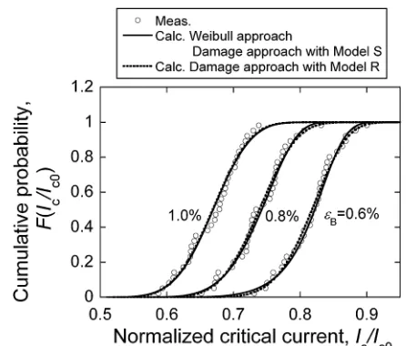
for analysis. The cumulative (F) and density (f) probability

of the critical current (Ic=Ic0) values at "B¼0:6, 0.8 and

1.0%, taken from Fig. 1(a), are presented in Figs. 2 and 3, respectively. The results shown in Figs. 2 and 3 were analyzed by the Weibull approach and the damage approach.

3. Procedure for Analysis

3.1 Description of the distribution of Ic=Ic0 values by

means of the Weibull approach

The three parameter Weibull distribution function has been proposed originally to describe the strength distribution

of materials.15)_{This function has been used to describe the}

transport critical current distribution11–14) _{and the critical}

current distribution at weak links for analysis ofV(voltage)–

I(current) curve near the transition from superconducting to

normal conductive state.16,17) _{The three-parameter Weibull}

distribution function is characterized by three parameters

(ðIc=Ic0Þmin is the minimum (lower limit) value of critical

current, ðIc=Ic0Þ0 is the scale parameter, and mis the shape

parameter). With these parameters, the cumulative

proba-bilityF of the critical current (Ic=Ic0) is expressed by

FðIc=Ic0Þ ¼1exp 1

Ic=Ic0 ðIc=Ic0Þmin

ðIc=Ic0Þ0

m

ð1Þ

The values of ðIc=Ic0Þmin, m and ðIc=Ic0Þ0 in eq. (1) which

describe the measured distributions at"B¼0:6, 0.8 and 1.0%

were estimated by the regression analysis, as shown in Section 4.1.

3.2 Description of the distribution of Ic=Ic0 values by

means of the damage approach

Figure 4(a) shows a micrograph of the transverse cross-section of the sample. When the thickness direction is enlarged by a factor of 3, the shape of the core (the region in which Bi2223 filaments are embedded in Ag) can be more clearly observed, as shown in Fig. 4(b).

Fig. 1 Variation of (a) normalized critical currentIc=Ic0and (b) coefficient

of variation (COV) ofIc=Ic0andIcvalues with increasing bending strain "B, measured for 33 specimens.10,11)

Fig. 2 Cumulative probability F of measured critical current Ic=Ic0 at "B¼0:6, 0.8 and 1.0%. Solid curves show the results analyzed using the

As the damage of the Bi2223 filaments existing in the core causes the reduction in critical current, it is necessary to formulate the shape. Taking the width- and

thickness-directions of the composite tape as the x- and y-axes,

respectively, and the center of the composite tape as x¼

y¼0 (Fig. 4(c)), and denoting the y-coordinate of the

boundary of the core as ycore, we formulated ycore as a

function of x in two models. One is the actual

shape-incorporated model with the core boundary ABCDEFGHA

in Fig. 4(c), which is referred to as Model S. This model is rigid but requires a relatively long time for calculation. Another model is used where the shape of the core is approximated as a rectangle (abcd in Fig. 4(c)); this model is referred to as Model R. This model is not rigid but is practical and simple to calculate; it gives a good approx-imation of the relation between critical current and damage front at high bending strains, as well as between critical current and bending strain, as shown later in Section 4.3.

3.2.1 Model S

In Model S, the actual shape of the core is used

(ABCDEFGHA in Fig. 4(c)), and the y-coordinate of the

boundary of the core, ycore, is expressed as a function of x

with a 9th order polynomial for the present sample.11,12)

The unit of length is millimeters.

ABC:ycore¼0:117324þ1:13901xþ10:0985x2þ38:6006x3þ83:9271x4

þ113:805x5þ97:9306x6þ51:8601x7þ15:3722x8þ1:94706x9

for 1:76<x<0:017 CDE: ycore¼0:0765863þ0:132501xþ1:36795x211:2465x3þ36:2954x4

63:3049x5þ64:1326x637:7293x7þ11:9598x81:58008x9

for 0:017<x<þ1:76

EFGHA: symmetry of rotation of ABCDE with respect tox¼y¼0

9 > > > > > > > > > > > = > > > > > > > > > > > ;

ð2Þ

Under the applied bending strain, tensile strain is exerted on the filaments in the core along the sample length direction (current transport direction). The exerted tensile strain is dependent on the location; it increases with distance from the

neutral axis.6,11,12)Accordingly, the filaments farthest from

the neutral axis, existing at ycore¼ycore,max (¼ycore,maxðSÞ

andycore,maxðRÞin Fig. 4(c) for Models S and R,

respective-ly), have the highest tensile strain and are fractured first at

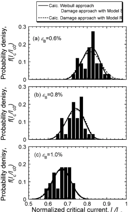
Fig. 3 Probability densityfof measured critical currentIc=Ic0at"B¼0:6,

0.8 and 1.0%. Solid curves show results analyzed using the direct Weibull approach and the damage approach with Model S, which were on the same curves. Broken curves show the calculation results from eq. (9) based on the damage approach with Model R.

(a)

(b)

(c)

Fig. 4 Transverse cross-section of the composite tape. (a) Optical micro-graph in the as-observed state and the shape of the core. (b) Deformed optical micrograph, where the thickness direction is expanded by a factor 3; broken curve shows the core boundary. (c) Schematic representation of the geometry of the cross-section in relation to the damage extension. Damage occurs first at the outermost filaments at the maximum value of

ycore(ycore,max) when the bending strain"Breaches the irreversible bending

strain"B,irr. When the bending strain"Bis raised from"B,irrto"B;iand then

"B¼"B,irr (the irreversible bending strain at which damage

first occurs and critical current reduction starts). When the

bending strain is raised from"B,irr to"B;i and then to"B;iþ1,

the damage frontyf extends downward fromycore,max toyf;i

and then toyf;iþ1(Fig. 4(c)). The damage extension leads to

reduction in the cross-sectional area of the current trans-porting Bi2223 filaments and therefore critical current.

Denoting the tensile fracture strain of the filaments under

no residual strain as"f and the residual strain of the filaments

along the sample length direction as"r, the damage frontyf

is given by11,12)

yf ¼

ðt=2Þð"f"rÞ

"B

ð3Þ

The first damage takes place at yf ¼ycore,max at"B¼"B,irr

as stated above. Substituting yf ¼ycore,max and "B¼"B,irr

into eq. (3), we obtain the irreversible bending strain "B,irr

in the following form:

"B,irr¼

t=2

ycore,max

ð"f"rÞ ð4Þ

Because the "f"r value is different from specimen to

specimen and also from position to position within a

specimen, the yf (eq. (3)) and "B,irr (eq. (4)) are distributed

among the specimens. The normalized critical currentIc=Ic0

is 1(unity) for"B"B,irr. For"B"B,irr, the damage frontyf

extends downward as stated above, leading to reduction in the cross-sectional area of the current transporting Bi2223 filaments and therefore critical current.

In the Bi2223 composite tape, only the tensile side is damaged up to around 1.0% bending strain, as has been

verified by the X-ray diffraction analysis.18) _{In the present}

work, we consider the case where only the core for y>0

(tensile side under the bending strain) is damaged. The experimental results are described for this condition, as shown later in Section 4.2. When all specimens are damaged

as in the present case (Ic=Ic0values of all specimens are less

than unity at"B¼0:6, 0.8 and 1.0% (Figs. 1, 2 and 3)), the

normalized critical current,Ic=Ic0, is expressed by11,12)

Ic

Ic0

¼1

Z

Wcore=2

Wcore=2

ðt=2Þ ycore

t=2 "f "r

"B

dx=Acore ð5Þ

where Acore (¼0:646mm2 in the present sample) is the

cross-sectional area of the core.

3.2.2 Model R

In Model R, the shape of the core is approximated as a rectangle (abcd in Fig. 4(c)). In this approximation, the

width of the core (Wcore ð¼3:52mmÞin Fig. 4(c)) and

cross-sectional area of the core (Acore¼0:646mm2) are taken to

be same as those of Model S. The x- and y-coordinates of

the boundary of the core, xcore and ycore, respectively, are

expressed by eq. (6).11)_{The unit of length is millimeters.}

ab:ycore¼0:0918for1:76x1:76

bc:xcore¼1:76for0:0918y0:0918

cd:ycore¼ 0:0918for1:76x1:76

da:xcore¼ 1:76for0:0918y0:0918

9 > > > = > > > ;

ð6Þ

The relations among"B,yf=ðt=2Þ,"f"r and"B,irr given by

eqs. (3) and (4) hold both for Models R and S. Due to the

simplification of the shape of the core in Model R, Ic=Ic0

(<1) expressed by eq. (5) for Model S is reduced to

Ic

Ic0

¼1

2 1þ

1

ycore,max=ðt=2Þ

"f"r

"B

ð7Þ

whereycore,max¼ycore,maxðRÞ ð¼0:0918mmÞ.

4. Results and Discussion

4.1 Analysis of the distribution of Ic=Ic0 values by the

Weibull approach

When ðIc=Ic0Þmin¼0 in eq. (1), the parameters to be

estimated by the regression analysis are reduced to two

(ðIc=Ic0Þ0 and m). Such a function has been called a

two-parameter Weibull function. In the case of two-two-parameter

Weibull function, the relation of lnlnð1FÞ1 tolnðIc=Ic0Þ

is linear. If the measured (Ic=Ic0) values obey the

three-parameter function (eq. (1) with ðIc=Ic0Þmin>0), the plot

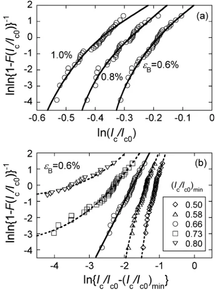
of lnlnð1FÞ1 against lnðIc=Ic0Þis convex.13) Figure 5(a)

shows the plot oflnlnð1FÞ1againstlnðIc=Ic0Þ, suggesting

that the distribution of theIc=Ic0values at"B¼0:6, 0.8 and

1.0% are described by the three-parameter Weibull

distribu-tion funcdistribu-tion withðIc=Ic0Þmin>0.

The values ofðIc=Ic0Þmin,mandðIc=Ic0Þ0that fit best to the

experimental result at each bending strain can be obtained by regression analysis in the following procedure. Taking the

data at"B¼0:6% as an example, the plot oflnlnð1FÞ1

Fig. 5 (a) Plot of lnlnð1FÞ1 against lnðIc=Ic0Þ for measured Ic=Ic0

values at"B¼0:6, 0.8 and 1.0%, which are upward convex. (b) Plot of

lnlnð1FÞ1againstlnfIc=Ic0 ðIc=Ic0Þmingfor variousðIc=Ic0Þminvalues

for measured Ic=Ic0 values at "B¼0:6%, as an example. The

lnlnð1FÞ1_lnfI

c=Ic0 ðIc=Ic0Þmingcurve is convex whenðIc=Ic0Þmin

is low (ðIc=Ic0Þmin¼0:50and 0.58) but is linear whenðIc=Ic0Þminis 0.66,

againstlnfIc=Ic0 ðIc=Ic0Þmingis convex when theðIc=Ic0Þmin

value is low (0.50, 0.58) but is concave when it is high (0.73, 0.80), as shown in Fig. 5(b). Between low and high values of

ðIc=Ic0Þmin, there exists a value of ðIc=Ic0Þmin that gives the

highest linearity for the relation betweenlnlnð1FÞ1 and

lnfIc=Ic0 ðIc=Ic0Þming, as shown by the case ofðIc=Ic0Þmin¼

0:66 in this example. Once this ðIc=Ic0Þmin value is

deter-mined, the values ofmandðIc=Ic0Þ0can be obtained from the

slope and extrapolation for the plot oflnlnð1FÞ1against

lnfIc=Ic0 ðIc=Ic0Þming.

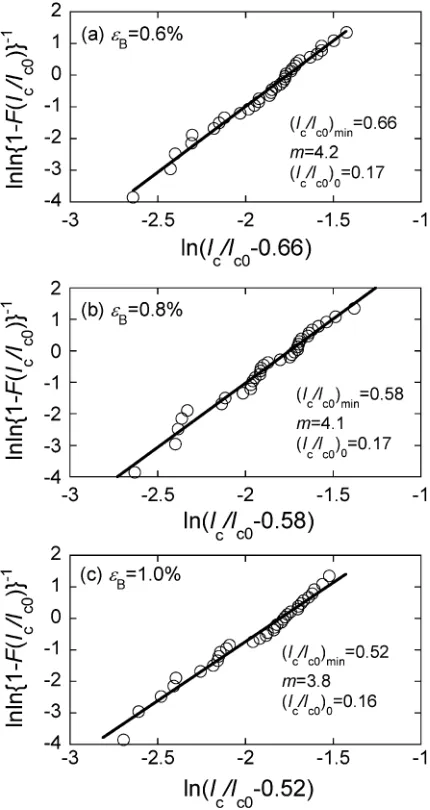
Figure 6 shows the plot of lnlnð1FÞ1 against lnfIc=

Ic0 ðIc=Ic0Þming, in which theðIc=Ic0Þminvalues that give the

highest linearity between the lnlnð1FÞ1 andlnfIc=Ic0

ðIc=Ic0Þming were 0.66, 0.58 and 0.52 at "B¼0:6, 0.8 and

1.0%, respectively. The high linearity between thelnlnð1

FÞ1andlnfIc=Ic0 ðIc=Ic0Þmingmeans that theIc=Ic0values

are described well by the three-parameter Weibull

distribu-tion funcdistribu-tion. The estimated values of fðIc=Ic0Þmin;m;

ðIc=Ic0Þ0gwere (0.66, 4.2, 0.17), (0.58, 4.1, 0.17) and (0.52,

3.8, 0.16) at"B¼0:6, 0.8 and 1.0%, respectively.

Substituting the estimated parameter values ofðIc=Ic0Þmin,

m and ðIc=Ic0Þ0 into eq. (1), the cumulative probability F–

critical currentIc=Ic0relations at"B¼0:6, 0.8 and 1.0% were

calculated, as shown by the solid curves in Fig. 2. The

measuredFIc=Ic0relations are well described. Moreover,

with the estimated parameter values, the cumulative proba-bility given by eq. (1) was converted to the density

probability f (frequency). The calculated fIc=Ic0relations

are presented as solid curves in Fig. 3, describing well the experimental results.

As shown above, it was found that the distribution ofIc=Ic0

values is described well by the three parameter Weibull distribution function. It should be noted that the decrease in

ðIc=Ic0Þmin with increasing bending strain "B, reflecting the

extension of the damage front of the most seriously damaged

specimen with increasing "B, could be estimated by the

Weibull approach quantitatively. However, the values of

Ic=Ic0, mandðIc=Ic0Þ0 were estimated as the fitting

param-eters at this stage. The physical meaning is discussed in Section 4.3.

4.2 Analysis of the distribution of Ic=Ic0 values by the

damage approach (Model S)

4.2.1 Estimation of distribution of"f "rvalues

If the distribution function of the"f"rvalues is known in

advance, the distribution of Ic=Ic0 can be calculated by

substitutingycore (eq. (2)), bending strain"Band the known

value ofAcore(0.646 mm2in the present sample) into eq. (5).

However, the"f"r value is not known in advance. In the

present work, using Model S in which the actual shape of the

core was incorporated, the "f"r values were

back-calcu-lated by substituting the following into eq. (5): the measured

Ic=Ic0values at each bending strain shown in Figs. 2 and 3,

theycoreexpressed by eq. (2), and the measured values of the

geometrical parameters (ycore,max¼ycore,maxðSÞ ¼0:117mm,

Wcore¼3:70mm,t¼0:270mm andAcore¼0:646mm2).

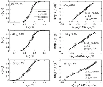
The cumulative probability F of the obtained "f"r

values at"B¼0:6, 0.8 and 1.0% are presented in Fig. 7(a),

(b), (c). The"f"rvalue corresponds to the tensile strain at

which the Bi2223 filaments in the composite tape fracture.

The average of "f"r value, ð"f"rÞave, was 0.25%. The

strain at which the filaments in the present composite tape are damaged under applied tensile strain has been estimated to be around 0.25% from the change in the stress carrying capacity upon occurrence of the damage in the stress-strain

curve.6,19) _{The estimated value ð"}

f"rÞave¼0:25% in the

present work coincides with this value.

The distribution of the obtained "f"r values was

formulated by application of the three-parameter Weibull distribution function, which has widely been used to describe

the strength distribution of materials.15) _{According to this}

function, the cumulative probability Fð"f"rÞ is expressed

by

Fð"f"rÞ ¼1exp

ð"f"rÞ ð"f"rÞmin

ð"f"rÞ0

m

ð8Þ

where ð"f"rÞmin is the minimum (lower limit) value of

"f"r, and ð"f"rÞ0 and m are the scale and shape

parameters, respectively. From the regression analysis, the

values of ð"f"rÞmin, ð"f "rÞ0 and m were estimated.

Fig. 6 Plot oflnlnð1FÞ1_againstlnfI

c=Ic0 ðIc=Ic0ÞmingforðIc=Ic0Þmin

values that give the highest linearity between lnlnð1FÞ1 and lnfIc=Ic0 ðIc=Ic0Þming. (ðIc=Ic0Þmin¼0:66, 0.58 and 0.52 at "B¼0:6,

Figure 7(a0_{), (b}0_{), (c}0_{) shows the plot oflnlnð1FÞ}1_against

lnf"f"r ð"f"rÞming, in which the ð"f"rÞmin values

that gave the highest linearity between lnlnð1FÞ1 and

lnf"f"r ð"f"rÞming were input. The high linearity

between lnlnð1FÞ1 _andlnf"

f"r ð"f"rÞming means

that the "f"r values are described well by the

three-parameter Weibull distribution function. The estimated

values of fð"f"rÞmin;m;ð"f"rÞ0g were (0.13%, 3.8,

0.14%), (0.094%, 3.9, 0.18%) and (0.022%, 3.8, 0.23%) at "B¼0:6, 0.8 and 1.0%, respectively. The solid curves in

Fig. 7(a), (b), (c) show the results of the regression analysis

corresponding to the solid lines in Fig. 7(a0_{), (b}0_{), (c}0_),

respectively.

4.2.2 Estimation of distribution ofIc=Ic0values using the

distributed"f "rvalues

By combining the distribution function of "f"r values

expressed by eq. (8) with eq. (5), and substituting ycore

(eq. (2)), the known values of t=2, Acore and "B, and the

estimated values of ð"f"rÞmin, m and ð"f"rÞ0, we

numerically calculated the cumulative (F) and density (f)

distributions of Ic=Ic0 at each bending strain. The

exper-imental results are reproduced well. It was confirmed that the present damage approach is a useful tool for reproduction of

distribution of Ic=Ic0 values with high accuracy. Note that

the calculation results were very close to the results of the Weibull approach shown with the solid curves in Figs. 2 and 3, and the difference between the damage approach and Weibull approach cannot be distinguished on this scale. This

means that (i) the distribution of"f"r values are estimated

accurately in the reverse analysis from distribution ofIc=Ic0

values to that of "f"r values through eq. (5) and (ii) the

critical current distribution of the Ic=Ic0 values obtained by

using the distributed"f"rvalues is expressed by the

three-parameter Weibull distribution as well as that obtained by the direct Weibull approach. An example demonstrating (i) and (ii) mentioned above is shown in Fig. 8. For comparison

with Fig. 5(b), this figure presents a plot of lnlnð1FÞ1

versus lnfIc=Ic0 ðIc=Ic0Þming for various ðIc=Ic0Þmin values

at "B¼0:6%, as calculated with the estimated distribution

function of "f "r values at "B¼0:6%. A linear relation

Fig. 7 Cumulative probability F of "f"r values at "B= (a) 0.6, (b) 0.8 and (c) 1.0%, and plot of lnlnð1FÞ1 against

lnf"f"r ð"f"rÞmingforð"f"rÞmin values that give the highest linearity betweenlnlnð1FÞ1and lnf"f"r ð"f"rÞming

(ð"f"rÞmin¼0:13, 0.094 and 0.022% at"B= (a0) 0.6, (b0) 0.8 and (c0) 1.0%, respectively).

Fig. 8 Plot oflnlnð1FÞ1 _againstlnfI

c=Ic0 ðIc=Ic0Þming for different ðIc=Ic0Þmin-values for distributedIc=Ic0values calculated by substituting

the distributed"f"rvalues into eq. (5).ðIc=Ic0Þminvalues used in this

the same as that in Fig. 5(b) is actually obtained for

ðIc=Ic0Þmin ¼0:66. The mand ðIc=Ic0Þ0 values are found to

be 4.2 and 0.17, respectively, for ðIc=Ic0Þmin¼0:66, which

are the same as those obtained by the direct Weibull approach shown in Fig. 6(a).

Here, the important finding is that the distribution function

of the measured damage-controlled Ic=Ic0 values, as

ex-pressed by the three-parameter Weibull distribution, can be reproduced accurately by the distribution of the

damage-controlling"f"r values, as expressed by the

three-param-eter Weibull distribution. This result suggests the followings. (a) The distribution of the critical current of bent-damaged specimens is accounted for from the viewpoint of the difference in damage evolution among the specimens. (b)

In the Weibull approach, the parameters ofðIc=Ic0Þmin,mand

ðIc=Ic0Þ0 were obtained as the fitting parameters, but the

physical significance was unknown. The correlation of the

distribution of Ic=Ic0 values to the distribution of "f"r

values obtained in the present work demonstrates that the parameters obtained by the Weibull approach surely reflect the difference in the damage extent among the specimens.

As shown above, using Model S for the damage approach,

we observed the correlation of distribution of"f"r values,

which are related to the distribution of the damage front

as indicated by eq. (3), to the distribution of Ic=Ic0 values.

However, if only the Model S is used, only numerical calculation can be conducted. Accordingly, it is difficult to

formulate a direct correlation of the distribution of "f"r

values to the distribution ofIc=Ic0values.

In the next sub-section, Model R is used for the damage

approach to find the correspondence of the ð"f"rÞmin, m

andð"f"rÞ0values (which characterize the distribution of

damage evolution), to theðIc=Ic0Þmin,mandðIc=Ic0Þ0 values

(which characterize the distribution of critical current).

4.3 Derivation of three parameter Weibull distribution

function forIc=Ic0values from the damage approach

using Model R

4.3.1 Difference and similarity inIc=Ic0 values between

Models S and R

In Model R, the shape of the core is approximated as a rectangle (Fig. 4(c)). The accuracy in calculation with this model is lower than that with Model S, in which the actual shape of the core is incorporated. In this subsection, the

difference and similarity in Ic=Ic0 values between Models S

and R are examined in advance of application of Model R.

When the "f"r value is known, the Ic=Ic0 at"B"B,irr

can be calculated by eqs. (5) and (7) for Models S and R,

respectively. "B,irr can be calculated using eq. (4) with

ycore,max=ðt=2Þ ¼0:87and 0.68 for Models S and R,

respec-tively. As the average of "f"r values, ð"f"rÞave, was

0.25%, the average irreversible bending strain "B,irr,ave is

calculated to be 0.29 and 0.37% for Models S and R, respectively. Figure 9 shows the calculated variation of

average ofIc=Ic0values,ðIc=Ic0Þave, for bending strain"B. The

calculated values of ðIc=Ic0Þave at "B¼0:6, 0.8 and 1.0%

calculated using Models S and R are almost the same, while

the values ofðIc=Ic0Þaveat lower bending strain differ between

the models (values of"B,irr,aveandðIc=Ic0Þaveat"B¼0:4% are

overestimated by Model R) due to the simplification of the

shape of the core in Model R. Because the critical current

Ic=Ic0at"B¼0:6, 0.8 and 1.0% is well expressed in a simple

form by eq. (7) in Model R, eq. (7) is used for formulation

of distribution ofIc=Ic0values at these high bending strains.

4.3.2 Derivation of distribution function ofIc=Ic0values

using Model R

TheIc=Ic0 for"B"B,irr expressed by eq. (7) in Model R

is dependent on the "f"r value, which is distributed

according to eq. (8). Substituting "f"r¼ f2ðIc=Ic0Þ

1g"Bfycore,maxðRÞ=ðt=2Þg derived from eq. (7) into eq. (8),

we have

FðIc=Ic0 at"BÞ

¼1exp

Ic=Ic0

1

2þ

ð"f "rÞmin=ð2"BÞ

ycore,maxðRÞ=ðt=2Þ

ð"f"rÞ0=ð2"BÞ

ycore,maxðRÞ=ðt=2Þ

8 > > > < > > > : 9 > > > = > > > ; m 2 6 6 6 4 3 7 7 7 5:

ð9Þ

In a comparison of eq. (9) with eq. (1), eq. (9) is simply a

form of the three parameter Weibull distribution for Ic=Ic0

values with the correspondence of

ðIc=Ic0Þmin¼

1 2þ

ð"f"rÞmin=ð2"BÞ

ycore,maxðRÞ=ðt=2Þ

ð10Þ

ðIc=Ic0Þ0¼

ð"f"rÞ0=ð2"BÞ

ycore,maxðRÞ=ðt=2Þ

ð11Þ

m(Ic=Ic0distribution)¼m("f"r distribution): ð12Þ

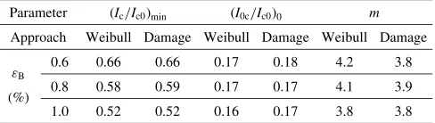
Substituting the parameter values of ð"f"rÞmin, ð"f"rÞ0

andmfor the"f"r distribution estimated by the statistical

analysis of "f"r values in the damage approach [fð"f

"rÞmin;m;ð"f"rÞ0g= (0.13%, 3.8, 0.14%), (0.094%, 3.9,

0.18%) and (0.022%, 3.8, 0.23%) at"B¼0:6, 0.8 and 1.0%,

respectively], and ycore,maxðRÞ=ðt=2Þ ¼0:68 into eqs. (10),

(11) and (12), we obtained the ðIc=Ic0Þmin, m and ðIc=Ic0Þ0

values for the distribution of Ic=Ic0 values, as shown in

Table 1. The parameter values calculated by the damage approach with Model R are almost the same as those estimated by the Weibull approach. A direct comparison

of the calculated cumulative probability F and probability

Fig. 9 Measured and analyzed change in average critical currentðIc=Ic0Þave

with bending strain "B. Results analyzed using Models S and R for ð"f"rÞave¼0:25% are shown as solid and broken curves, respectively.

Average irreversible bending strains ("B,irr,ave) analyzed using Models S

density f ofIc=Ic0values using eq. (9) based on the damage

approach using Model R with the measured ones is shown in Figs. 2 and 3, where the calculation results are presented

as broken curves. As shown above, the calculatedFðIc=Ic0Þ

(and fðIc=Ic0Þ) curves based on the damage approach with

Model S and direct Weibull approach are similar and the difference between them cannot be distinguished. The experimental results are described well also by the damage

approach with Model R. The slight difference at lower "B

(0.6 and 0.8%) between the damage approach with Model S (and the Weibull approach) and the damage approach with Model R stems from the simplification of the shape of the core in Model R.

It is important to note that the value ofmfor distribution of

Ic=Ic0is the same as that for the distribution of"f"rvalues

(eq. (12)) in Model R. "f"r refers to the tensile fracture

strain in the core of the Bi2223 filaments. The value ofmis

a measure of the coefficient of variation of the Ic=Ic0

ðIc=Ic0Þminas well as that of"f"r ð"f"rÞmin; for smaller

m, the distribution of the values of Ic=Ic0 ðIc=Ic0Þmin and

"f"r ð"f"rÞminis smaller. Equation (12) indicates that

the coefficient of variation of the normalized critical current distribution is governed by the difference in damage evolution among the specimens stemming from the

distri-buted "f"r values. As the distribution of "f"r values

follows the three-parameter Weibull distribution, the Ic=Ic0

values also follows the same type distribution function. In

this way, the reason why the distribution ofIc=Ic0values of

bent-damaged specimens is described by the three-parameter Weibull distribution function is accounted for by the differ-ence in damage evolution among the specimens.

5. Conclusions

(1) The distribution of the measured normalized critical current values of the Bi2223 composite tape (VAM1 sample) bent by 0.6, 0.8 and 1.0% in a round robin test of VAMAS/TWA16 were described by the three-parameter Weibull distribution function.

(2) The distribution of the measured normalized critical current values was also described well by the damage evolution approach, in which the difference in damage evolution among the specimens was correlated to the distribution critical current values. From this approach,

the Weibull distribution function for critical current values was derived, which gave almost the same parameter values of minimum critical current, scale parameter and shape parameter as those obtained by the direct application of the Weibull distribution function to the experimental results.

(3) Based on the results (1) and (2) above, the reason why the normalized critical current values of bent-damaged composite tape is described by the three-parameter Weibull distribution function was accounted for in a quantitative manner by the difference in damage evolution among the specimens.

Acknowledgement

The authors wish to express their gratitude to The Ministry of Education, Culture, Sports, Science and Technology, Japan, for a grant-in-aid for scientific research.

REFERENCES

1) H. Kitaguchi, K. Itoh, H. Kumakura, T. Takeuchi, K. Togano and H. Wada: IEEE Trans. Appl. Supercond.11(2001) 3058–3061. 2) R. Passerini, M. Dhalle’, E. Giannini, G. Witz, B. Seeber and R.

Flu¨kiger: Physica C371(2002) 173–184.

3) H. W. Weijers, J. Schwartz and B. ten Haken: Physica C372–376 (2002) 1364–1367.

4) K. Osamura, M. Sugano and K. Matsumoto: Supercond. Sci. Technol. 16(2003) 971–975.

5) H. S. Shin and K. Katagiri: Supercond. Sci. Technol.16(2003) 1012– 1018.

6) S. Ochiai, T. Matsuoka, J. K. Shin, H. Okuda, M. Sugano, M. Hojo and K. Osamura: Supercond. Sci. Technol.20(2007) 1076–1083. 7) S. Ochiai, J. K. Shin, S. Iwamoto, H. Okuda, S. S. Oh, D. W. Ha and

M. Sato: J. Appl. Phys.103(2008) 123911 (8 pp).

8) S. Ochiai, H. Rokkaku, J. K. Shin, S. Iwamoto, H. Okuda, K. Osamura, M. Sato, A. Otto and A. Malozemoff: Supercond. Sci. Technol.21 (2008) 075009 (13pp).

9) K. Katagiri, H. S. Shin, K. Kasaba, T. Tsukinokizawa, K. Hiroi, T. Kuroda, K. Itoh and H. Wada: Supercond. Sci. Technol.16(2003) 995– 999.

10) T. Kuroda,et al.: Physica C425(2005) 111–120.

11) S. Ochiai, J. K. Shin, H. Okuda, M. Sugano, M. Hojo, K. Osamura, T. Kuroda, K. Itoh and H. Wada: Supercond. Sci. Tecnol.21 (2008) 054002 (14pp).

12) S. Ochiai, H. Okuda, M. Sugano, M. Hojo, K. Osamura, T. Kuroda, K. Itoh, H. Kitaguchi, H. Kumakura and H. Wada: Supercond. Sci. Technol.23(2010) 025006 (12 pp).

13) S. Ochiai, M. Fujimoto, H. Okuda, S. S. Oh and D. W. Ha: J. Appl. Phys.105(2009) 06912 (8pp).

14) S. Ochiai, M. Fujimoto, J. K. Shin, H. Okuda, S. S. Oh and D. W. Ha: J. Appl. Phys.106(2009) 103916 (11 pp).

15) W. Weibull: J. Appl. Mech.28(1951) 293–297.

16) T. Kiss, T. Matsushita and F. Irie: Supercond. Sci. Technol.12(1999) 1079–1082.

17) M. Ahoranta, J. Lehtonen, P. Kova´cˇ, I. Husˇek and T. Melisˇek: Physica C401(2004) 241–245.

18) H. Okuda, J. K. Shin, S. Iwamoto, K. Morishita, Y. Mukai, H. Matsubayashi, S. Ochiai, A. Otto, E. J. Harley, A. Malozemoff and M. Sato: Scr. Mater.58(2008) 687–690.

19) S. Ochiai, H. Okuda, M. Sugano, M. Hojo and K. Osamura: J. Appl. Phys.107(2010) 083904 (9pp).

Table 1 Estimated values ofðIc=Ic0Þmin,I0andmfrom the direct Weibull

approach and damage approach with Model R (eq. (9)) at"B¼0:6, 0.8

and 1.0%.

Parameter ðIc=Ic0Þmin ðI0c=Ic0Þ0 m

Approach Weibull Damage Weibull Damage Weibull Damage

"B

0.6 0.66 0.66 0.17 0.18 4.2 3.8